Basic Overview

Using common lib (pandas_datareader, datetime, matplotlib & numpy) to visualize companies listed on stock exchange.

In this illustration, I am going to compare 3 different S&P 500 ETFs with tickers namely SPY, VOO & IVV

Installation

Use the package manager pip to install pandas_datareader (If you haven't already).

python -m pip install pandas_datareader

Quick start

Import required libs as usual.

import pandas_datareader.data as web
import datetime
import matplotlib.pyplot as plt
import numpy as np

Assign the start and end date (I chose 10 years period for illustration).

start_date = datetime.datetime(2012,4,12)
end_date = datetime.datetime(2022,5,12)

Source required data from Yahoo for the specified dates for all the 3 tickers, and return only top 5 results for ticker SPY.

spy = web.DataReader("SPY",'yahoo',start_date,end_date)
voo = web.DataReader("VOO",'yahoo',start_date,end_date)
ivv = web.DataReader("IVV",'yahoo',start_date,end_date)
spy.head()

Plot for ticker SPY for "Open", "Close", "High", "Low" on the same axis for specified time period.

spy["Open"].plot(label='Open',figsize = (16,8))
spy["Close"].plot(label='Close')
spy["High"].plot(label='High')
spy["Low"].plot(label='Low')
plt.title('Price Changes for S&P 500 ETF over 10-year period')
plt.ylabel('Price ($)')
plt.legend()
plt.show()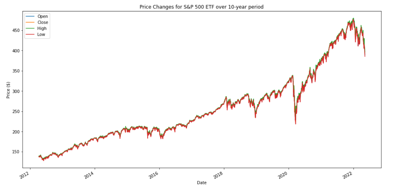

Comparing "Close" price for ticker SPY, VOO, IVV on same axis for specified time period.

spy['Close'].plot(label = 'SPY Close',figsize = (16,8),color ='black')
voo['Close'].plot(label = 'VOO Close')
ivv['Close'].plot(label = 'IVV Close')
plt.xlabel('Year')
plt.ylabel('Price ($)')
plt.title('Price Changes for SPY, VOO & IVV ETF over 10-year period')
plt.legend()
plt.show()

Comparing "Volume" traded for ticker SPY, VOO, IVV on same axis for specified time period.

spy['Volume'].plot(label = 'SPY',figsize = (16,8))
voo['Volume'].plot(label = 'VOO')
ivv['Volume'].plot(label = 'IVV')
plt.xlabel('Year')
plt.ylabel('Volume')
plt.legend()
plt.show()

Comparing "MA50", "MA100", "MA200" traded for ticker SPY on same axis for specified time period. *MA stands for Moving Average

spy['Close'].plot(label = 'SPY (S&P 500)',figsize = (18,9))
spy['MA50'] = spy['Close'].rolling(50).mean()
spy['MA50'].plot(label = 'MA 50')
spy['MA100'] = spy['Close'].rolling(100).mean()
spy['MA100'].plot(label = 'MA 100')
spy['MA200'] = spy['Close'].rolling(200).mean()
spy['MA200'].plot(label = 'MA 200')
plt.xlabel('Year')
plt.ylabel('Price')
plt.title('SPY (S&P 500) ETF MA 50, 100 & 200 over 10 years period')
plt.legend()
plt.show()

Obtaining daily percentage change (close price) for ticker SPY, VOO, IVV and return only top 5 results for specified time period.

spy['Returns'] = (spy['Close']/spy['Close'].shift(1))-1
voo['Returns'] = (voo['Close']/voo['Close'].shift(1))-1
ivv['Returns'] = (ivv['Close']/ivv['Close'].shift(1))-1
spy.head()

Obtaining (KDE) Kernel Density Estimate of Returns for ticker SPY, VOO, IVV.

spy['Returns'].plot(kind ='kde',label='spy',figsize = (10,5))
voo['Returns'].plot(kind ='kde',label='voo')
ivv['Returns'].plot(kind ='kde',label='ivv')
plt.legend()

Things that are still lacking

Cumulative Return, Market Cap Plot, and any other relevant.

Contributing

Pull requests are welcome. For major changes, please open an issue first to discuss what you would like to change.

Please make sure to update tests as appropriate.

Special thanks for guidance

Ahmad Bazzi