ultrasphere-harmonics

---

Documentation: https://ultrasphere-harmonics.readthedocs.io

Source Code: https://github.com/ultrasphere-dev/ultrasphere-harmonics

---

Hyperspherical harmonics in NumPy / PyTorch

Installation

Install this via pip (or your favourite package manager):

pip install ultrasphere-harmonics[cli]

Usage

All functions support batch calculation.

Following Generalized universal function API (NumPy), Batch dimensions are mapped to the first dimensions of arrays and Core dimensions are mapped to the last dimensions of arrays.

Spherical Harmonics

>>> from array_api_compat import numpy as np
>>> from ultrasphere import create_spherical
>>> from ultrasphere_harmonics import harmonics
>>> harm = harmonics( # flattened output
...     create_spherical(), # structure for spherical coordinates
...     {"theta": np.asarray(0.5), "phi": np.asarray(1.0)}, # spherical coordinates
...     n_end=2, # maximum degree - 1
...     phase=0 # the phase convention (see below for details)
... )
>>> np.round(harm, 2)
array([0.28+0.j  , 0.43+0.j  , 0.09+0.14j, 0.09-0.14j])

Batch calculation

>>> harm = harmonics( # flattened output
...     create_spherical(), # structure for spherical coordinates
...     {"theta": np.asarray([0.5, 0.6]), "phi": np.asarray([1.0])}, # spherical coordinates
...     n_end=2, # maximum degree - 1
...     phase=0 # the phase convention (see below for details)
... )
>>> np.round(harm, 2)
array([[0.28+0.j  , 0.43+0.j  , 0.09+0.14j, 0.09-0.14j],
       [0.28+0.j  , 0.4 +0.j  , 0.11+0.16j, 0.11-0.16j]])

Hyperspherical Harmonics

Spherical harmonics for higher dimensions or lower dimensions can be calculated by specifying the structure of Vilenkin–Kuznetsov–Smorodinsky (VKS) polyspherical coordinates.

>>> from ultrasphere import create_standard
>>> harm = harmonics( # flattened output
...     create_standard(4), # structure for spherical coordinates
...     {"theta0": np.asarray(0.5), "theta1": np.asarray(0.75), "theta2": np.asarray(1.0), "theta3": np.asarray(1.25)}, # spherical coordinates
...     n_end=2, # maximum degree - 1
...     phase=0 # the phase convention (see below for details)
... )
>>> np.round(harm, 2)
array([0.19+0.j  , 0.38+0.j  , 0.15+0.j  , 0.08+0.j  , 0.03+0.08j,
       0.03-0.08j])

The definition and notation of VKS polyspherical coordinates follows [Cohl2012, Appendix B]. See ultrasphere for details of the coordinates.

The definition of (hyper)spherical harmonics also follows [Cohl2012, Appendix B] if phase=Phase(0) is set, which would be described later.

• [Cohl2012] Cohl, H. (2012). Fourier, Gegenbauer and Jacobi Expansions for a Power-Law Fundamental Solution of the Polyharmonic Equation and Polyspherical Addition Theorems. Symmetry, Integrability and Geometry: Methods and Applications (SIGMA), 9. https://doi.org/10.3842/SIGMA.2013.042

Expansion and Evaluation

Expansion

>>> from ultrasphere_harmonics import expand, expand_evaluate
>>> def my_function(spherical):
...     return np.sin(spherical["theta"]) + np.cos(spherical["phi"])
>>> expansion_coef = expand(
...     create_spherical(),
...     my_function,
...     n_end=6, # maximum degree - 1
...     n=12, # number of points for numerical integration
...     does_f_support_separation_of_variables=False,
...     phase=0,
...     xp=np
... )
>>> np.round(expansion_coef, 2) + 0.0
array([ 2.78+0.j,  0.  +0.j,  1.71+0.j,  1.71+0.j, -0.78+0.j,  0.  +0.j,
        0.  +0.j,  0.  +0.j,  0.  +0.j,  0.  +0.j,  0.4 +0.j,  0.  +0.j,
        0.  +0.j,  0.  +0.j,  0.  +0.j,  0.4 +0.j, -0.13+0.j,  0.  +0.j,
        0.  +0.j,  0.  +0.j,  0.  +0.j,  0.  +0.j,  0.  +0.j,  0.  +0.j,
        0.  +0.j,  0.  +0.j,  0.2 +0.j,  0.  +0.j,  0.  +0.j,  0.  +0.j,
        0.  +0.j,  0.  +0.j,  0.  +0.j,  0.  +0.j,  0.  +0.j,  0.2 +0.j])

Evaluation

>>> spherical = {
...     "theta": np.asarray(0.5),
...     "phi": np.asarray(0.75),
... }
>>> my_function_expected = my_function(spherical)
>>> np.round(my_function_expected, 6)
np.float64(1.211114)
>>> my_function_approx = expand_evaluate(
...     create_spherical(),
...     expansion_coef,
...     spherical,
...     phase=0
... )
>>> np.round(my_function_approx, 6)
np.complex128(1.248959+0j)

See API Reference for further details and examples.

2 formats for storing spherical harmonics

Format	indexing (n, m) in type ba coordinates
Multidimensional	array[..., n, m]
Flatten	array[..., (n - 1) ** 2 + (m % (2 * n - 1))]

Advantages of Multidimensional format

• Easy to understand and use
• Easy to slice
• Summantion over specific quantum number is easy

Advantages of Flatten format

• Memory efficient
• Easy to use linear algebra functions like np.linalg.solve, np.inv etc.
• Summation over all quantum numbers is easy

The format can be converted using flatten_harmonics() and unflatten_harmonics() functions.

4 different definitions of spherical harmonics for type ba coordinates

There are 4 different definitions of spherical harmonics in the literature. This package supports all of them by changing phase parameter.

Associated Legendre Polynomial

The associated Legendre polynomial is defined as follows:

$$ P_n^m (x) = (1 - x^2)^{\frac{m}{2}} \frac{d^m}{dx^m} P_n (x) $$

In some literature, the Condon-Shortley phase $(-1)^m$ is included in the definition of $P_n^m$ as follows:

$$ {P'}_n^m (x) = (-1)^m (1 - x^2)^{\frac{m}{2}} \frac{d^m}{dx^m} P_n (x) $$

Spherical Harmonics

phase	definition	difference from Phase(0)	Used in (for example)
Phase(0)	$Y_n^{(0),m} = \sqrt{\frac{2n+1}{4\pi} \frac{(n-|m|)!}{(n+|m|)!}} P_n^{|m|} (\cos \theta) e^{i m \phi}$	$1$	[Kress2014]
Phase(1)	$Y_n^{(1),m} = \sqrt{\frac{2n+1}{4\pi} \frac{(n-m)!}{(n+m)!}} P_n^m (\cos \theta) e^{i m \phi}$	$(-1)^{\frac{|m| - m}{2}}$	Wolfram MathWorld
Phase(2)	$Y_n^{(2),m} = (-1)^m \sqrt{\frac{2n+1}{4\pi} \frac{(n-|m|)!}{(n+|m|)!}} P_n^{|m|} (\cos \theta) e^{i m \phi}$	$(-1)^m$	[Gumerov2004]
Phase(3)	$Y_n^{(3),m} = (-1)^m \sqrt{\frac{2n+1}{4\pi} \frac{(n-m)!}{(n+m)!}} P_n^m (\cos \theta) e^{i m \phi}$	$(-1)^{\frac{|m| + m}{2}}$	Scipy

Note that $\forall m \in \mathbb{Z}. (-1)^m = (-1)^{-m}$ holds.

The Phase parameter would have less meaning for hyperspherical harmonics, but it is kept for consistency. The phase convention is applied to all type a nodes in the VKS polyspherical coordinates.

• [Gumerov2004]: Gumerov, N. A., & Duraiswami, R. (2004). Recursions for the Computation of Multipole Translation and Rotation Coefficients for the 3-D Helmholtz Equation. SIAM Journal on Scientific Computing, 25(4), 1344–1381. https://doi.org/10.1137/S1064827501399705
• [Kress2014]: Kress, R. (2014). Linear Integral Equations (Vol. 82). Springer New York. https://doi.org/10.1007/978-1-4614-9593-2

Demonstration

Scattering by a sound-soft sphere in $\mathbb{R}^d, d \geq 2$

Mathematical formulation

Let $d \in \mathbb{N} \setminus \lbrace 1 \rbrace$ be the dimension of the space, $k$ be the wave number, and $\mathbb{S}^{d-1} = \lbrace x \in \mathbb{R}^d \mid |x| = 1 \rbrace$ be a unit sphere in $\mathbb{R}^d$.

Asuume that $u_\text{in}$ is an incident wave satisfying the Helmholtz equation

$$ \Delta u_\text{in} + k^2 u_\text{in} = 0 $$

and scattered wave $u$ satisfies the following:

$$ \begin{cases} \Delta u + k^2 u = 0 \quad &x \in \mathbb{R}^d \setminus \overline{\mathbb{S}^{d-1}} \\ u = -u_\text{in} \quad &x \in \mathbb{S}^{d-1} \\ \lim_{|x| \to \infty} |x|^{\frac{d-1}{2}} \left( \frac{\partial u}{\partial |x|} - i k u \right) = 0 \quad &\frac{x}{|x|} \in \mathbb{S}^{d-1} \end{cases} $$

The total wave $u_\text{tot}$ is defined as follows:

$$ u_\text{tot} = u_\text{in} + u $$

Let $N \in \mathbb{N}$ be the truncation number for the spherical harmonics expansion.

Then $u$ can be approximated as follows:

$$ u(x) = - \sum_{n=0}^{N-1} \sum_{p=1}^{N(d,n)} \left(u_\text{in}\right)_{n, p} \frac{h^{(1)} (k |x|) Y_{n,p} \left( \frac{x}{|x|} \right)}{h^{(1)} (k)} $$

where

$$ \left(u_\text{in}\right)_{n, p} := \sum_{i} w_i u_\text{in} (x_i) \overline{Y_{n,p}(x_i)} \approx \int_{\mathbb{S}^{d-1}} u_\text{in}(x) \overline{Y_{n,p}(x)} d x $$

and $\lbrace(x_i, w_i)\rbrace_i$ are the quadrature points and weights.

Functions needed

• expand(): to compute $\left(u_\text{in}\right)_{n, p}$
• harmonics_regular_singular(): to compute $h^{(1)} (k |x|) Y_{n,p} \left( \frac{x}{|x|} \right)$
• ultrasphere.shn1(): to compute $h^{(1)} (k)$
• xp.sum(): to compute the summation

Implementation

See src/ultrasphere_harmonics/cli.py. The code works for any spherical coordinates (dimension-independent).

Results

The incident wave is set to be a spherical wave emitted from the point $x_0 := (2, 0, \ldots, 0)$:

$$ u_\text{in} (x) = h^{(1)} (k |x - x_0|) $$

• --k: set the wave number $k$
• --n-end: set the truncation number $N$

The three waves $u_\text{in}, u, u_\text{tot}$ in $[-3, 3] \times [-3, 3] \times \lbrace 0 \rbrace^{d-2}$ are plotted.

2D example (type a coordinates):

uv run ultrasphere-harmonics scattering a --k 10 --n-end 20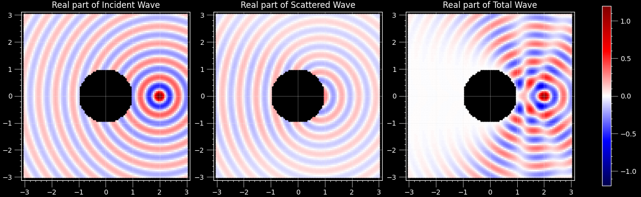

3D example (type ba coordinates):

uv run ultrasphere-harmonics scattering ba --k 10 --n-end 20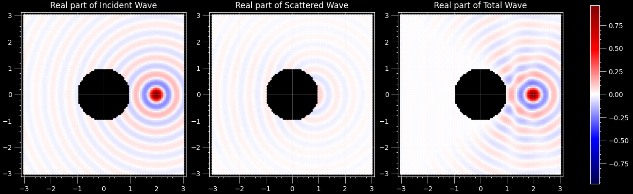

4D example (type bba coordinates):

uv run ultrasphere-harmonics scattering bba --k 1 --n-end 5

4D example (type caa coordinates):

uv run ultrasphere-harmonics scattering caa --k 1 --n-end 5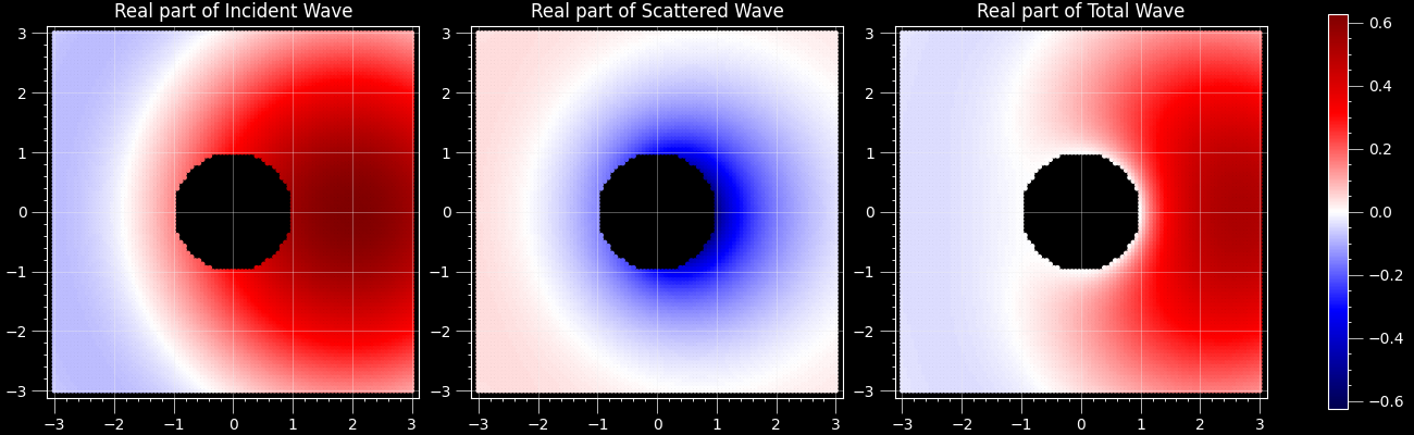

One can see that the total wave (right) is close to zero (white) near the sphere (circle) in all cases.

Spherical Harmonics Expansion of Stanford Bunny

A ray is emitted from a certain point to each direction on a 3D unit sphere and the distance to the most far intersection point is measured.

Directions are randomly sampled in $\mathbb{S}^2$ and the approximated radius are plotted.

uv run ultrasphere-harmonics expand-bunny

Hyperspherical Harmonics Expansion of voxelated 3D Stanford Bunny projected onto 4D Sphere

A ray is emitted from a certain point to each direction on a 3D unit sphere and the points before the most far intersection point are treated as 1 and the others are treated as 0. The shape is projected onto a 4D unit sphere using stereographic projection and expanded using hyperspherical harmonics and quadrature on a 4D unit sphere, using the similar method as in [Bonvallet2007] and [Hosseinbor2013]. (Not identical, as Least-squares method is not used here to make it simpler, etc.)

Points are randomly sampled in $[-1, 1]^3$ and points are plotted if and only if the approximated radius is greater than threshold which defaults to 0.5.

uv run ultrasphere-harmonics expand-bunny-4d

References

• [Bonvallet2007]: Bonvallet, B., Griffin, N., & Li, J. (2007). A 3D shape descriptor: 4D hyperspherical harmonics “an exploration into the fourth dimension.” Proceedings of the IASTED International Conference on Graphics and Visualization in Engineering, 113–116.
• [Hosseinbor2013]: Hosseinbor, A. P., Chung, M. K., Schaefer, S. M., van Reekum, C. M., Peschke-Schmitz, L., Sutterer, M., Alexander, A. L., & Davidson, R. J. (2013). 4D Hyperspherical Harmonic (HyperSPHARM) Representation of Multiple Disconnected Brain Subcortical Structures. Medical Image Computing and Computer-Assisted Intervention : MICCAI ... International Conference on Medical Image Computing and Computer-Assisted Intervention, 16(0 1), 598–605. https://doi.org/10.1007/978-3-642-40811-3_75

Contributors ✨

Thanks goes to these wonderful people (emoji key):

This project follows the all-contributors specification. Contributions of any kind welcome!

Credits

This package was created with Copier and the browniebroke/pypackage-template project template.

The code examples in the documentation and docstrings are automatically tested as doctests using Sybil.