You are a junior data analyst working in the marketing analyst team at Cyclistic, a bike-share company in Chicago. The director of marketing believes the company’s future success depends on maximizing the number of annual memberships. Therefore, your team wants to understand how casual riders and annual members use Cyclistic bikes differently. From these insights, your team will design a new marketing strategy to convert casual riders into annual members. But first, Cyclistic executives must approve your recommendations, so they must be backed up with compelling data insights and professional data visualizations.
- The goals to strategize converting casual riders into annual members
- Understand how annual members and casual riders differ
- Analyzing the Cyclistic historical bike trip data to identify trends
- Design a new marketing strategy to convert casual riders into annual members
install.packages("tidyverse")
install.packages("dplyr")
install.packages("lubridate")
install.packages("ggplot2")

library(tidyverse)
library(lubridate)
library(ggplot2)
library(dplyr)
It's size are >25 MB so i can't upload it here
Note: The datasets have a different name because Cyclistic is a fictional company. For the purposes of this case study,
the datasets are appropriate and will enable you to answer the business questions. The data has been made available by
Motivate International Inc. under this license.
Data used :
- 2021, Month of 01-11
- 2022, Month of 01
Changes made :
- Mixing the 2021 and 2022 due to too many invalid data on 2021 month of 06-10, at the "started at" & "ended at" column's rows filled with "######".
- Cleaning and Aggregate all of each month files into one file named "202102-202201_divvy-tripdata.csv"
- Added "ride_length" & "day_of_week" columns using "Google Spreadsheet'
# Storing data to data frame
master_trip<- read.csv("202102-202201_divvy-tripdata.csv")


# Checking the columns and structure
colnames(master_trip)
str(master_trip)

# Making sure the categories & members are unique
ride_ctg <- unique(master_trip$rideable_type)
member_cat <- unique(master_trip$member_casual)
ride_ctg
member_cat
table(master_trip$rideable_type)
table(master_trip$member_casual)
master_trip$date <- as.Date(master_trip$started_at)
master_trip$day <- format(as.Date(master_trip$started_at), "%d")
master_trip$month <- format(as.Date(master_trip$started_at), "%m")
master_trip$year <- format(as.Date(master_trip$started_at), "%Y")
master_trip$day_of_week <- format(as.Date(master_trip$started_at), "%A")
master_trip$ride_length_mins <- difftime(master_trip$ended_at, master_trip$started_at, units = "mins")
master_trip$ride_length_mins <- as.numeric(as.character(master_trip$ride_length_mins))
Keeping the old data frame and creating a new data frame filled with cleaned data
master_trip_2 <- master_trip[!(master_trip$ride_length<=0),]
sum(master_trip$ride_length<=0)
sum(master_trip_2$ride_length<=0)
sum(master_trip$ride_length>=1440)
master_trip_2 <- master_trip_2[!(master_trip_2$ride_length>=1440),]
sum(master_trip_2$ride_length>=1440)
Summary :
- <= 0 mins ride_length removed, 1
- more than 1 day ride_length removed, 2
[1] "ride_id"            "rideable_type"      "started_at"         "ended_at"           "start_station_name"
[6] "start_station_id"   "end_station_name"   "end_station_id"     "start_lat"          "start_lng"
[11] "end_lat"            "end_lng"            "member_casual"      "ride_length"        "day_of_week"
[16] "X"                  "X.1"                "X.2"                "date"               "day"
[21] "month"              "year"               "ride_length_mins"
mean(master_trip_2$ride_length_mins)
median(master_trip_2$ride_length_mins)
min(master_trip_2$ride_length_mins)
max(master_trip_2$ride_length_mins)
Result :
- Mean : 19.44
- Median : 11.95
- Min : 0.01
- Max : 1439.95
# Mean - Casual : 26.84 | Member : 13.36
aggregate(master_trip_2$ride_length_mins~ master_trip_2$member_casual, FUN = mean)

# Median - Casual : 15.93 | Member : 9.55
aggregate(master_trip_2$ride_length_mins~ master_trip_2$member_casual, FUN = median)

# Min - Casual : 0.01 | Member : 0.01
aggregate(master_trip_2$ride_length_mins~ master_trip_2$member_casual, FUN = min)

# Max - Casual : 1439.91 | Member : 1439.95
aggregate(master_trip_2$ride_length_mins~ master_trip_2$member_casual, FUN = max)
master_trip_2$day_of_week <- ordered(master_trip_2$day_of_week, levels
= c("Sunday","Monday","Tuesday","Wednesday","Thursday","Friday","Saturday"))
aggregate(master_trip_2$ride_length_mins ~ master_trip_2$member_casual + master_trip_2$day_of_week, FUN =mean)
# Result
1                       casual                    Sunday                       31.05807
2                       member                    Sunday                       15.27465
3                       casual                    Monday                       27.21924
4                       member                    Monday                       12.94730
5                       casual                   Tuesday                       24.45944
6                       member                   Tuesday                       12.59973
7                       casual                 Wednesday                       23.24978
8                       member                 Wednesday                       12.61532
9                       casual                  Thursday                       23.13469
10                      member                  Thursday                       12.54225
11                      casual                    Friday                       24.92553
12                      member                    Friday                       13.08549
13                      casual                  Saturday                       29.15350
14                      member                  Saturday                       14.93197
master_trip_2 %>%
mutate(weekday = wday(started_at, label = TRUE)) %>%
group_by(member_casual, weekday) %>%
summarise(number_of_rides = n(), average_duration = mean(ride_length_mins)) %>%
arrange(member_casual, weekday)
# Result
 1 casual        Sun              479898             31.1
 2 casual        Mon              286263             27.2
 3 casual        Tue              274541             24.5
 4 casual        Wed              278868             23.2
 5 casual        Thu              285859             23.1
 6 casual        Fri              363154             24.9
 7 casual        Sat              556914             29.2
 8 member        Sun              376111             15.3
 9 member        Mon              418351             12.9
10 member        Tue              468600             12.6
11 member        Wed              478644             12.6
12 member        Thu              453470             12.5
13 member        Fri              445023             13.1
14 member        Sat              431584             14.9
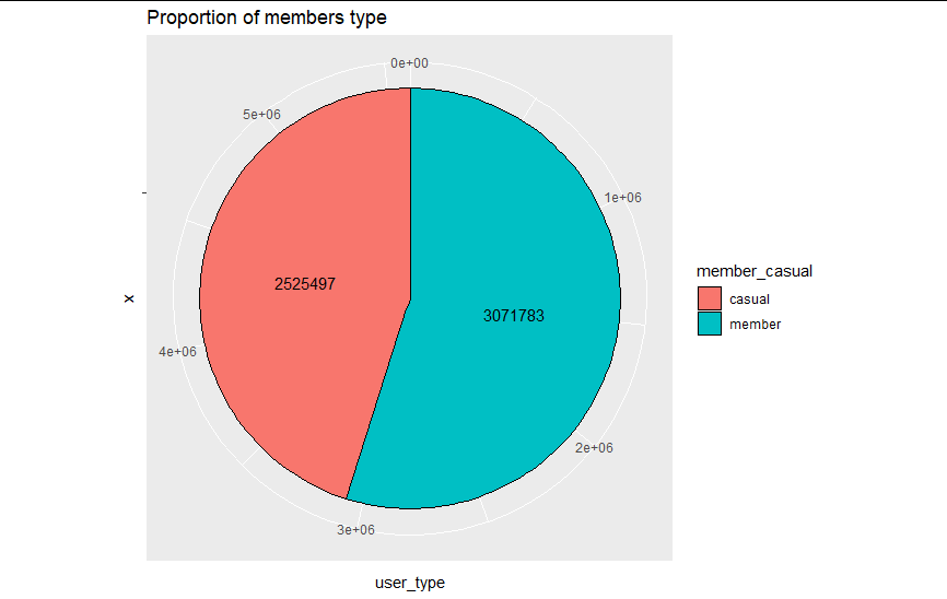
master_trip_2%>%
group_by(member_casual) %>%
summarise(user_type = n()) %>%
ggplot(aes(x="", y=user_type, fill=member_casual)) +
geom_col(color = "black") +
geom_text(aes(label = user_type), position = position_stack(vjust = 0.5),
            show.legend = FALSE) +
coord_polar(theta = "y")+
labs(title = "Proportion of members type")
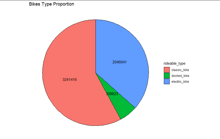
master_trip_2%>%
group_by(rideable_type) %>%
summarise(number_of_bikes = n()) %>%
ggplot(aes(x="", y=number_of_bikes, fill=rideable_type)) +
geom_col(color = "black") +
geom_text(aes(label = number_of_bikes), position = position_stack(vjust = 0.5),
show.legend = FALSE) +
coord_polar(theta = "y") +
theme_void() +
labs(title = "Bikes Type Proportion")
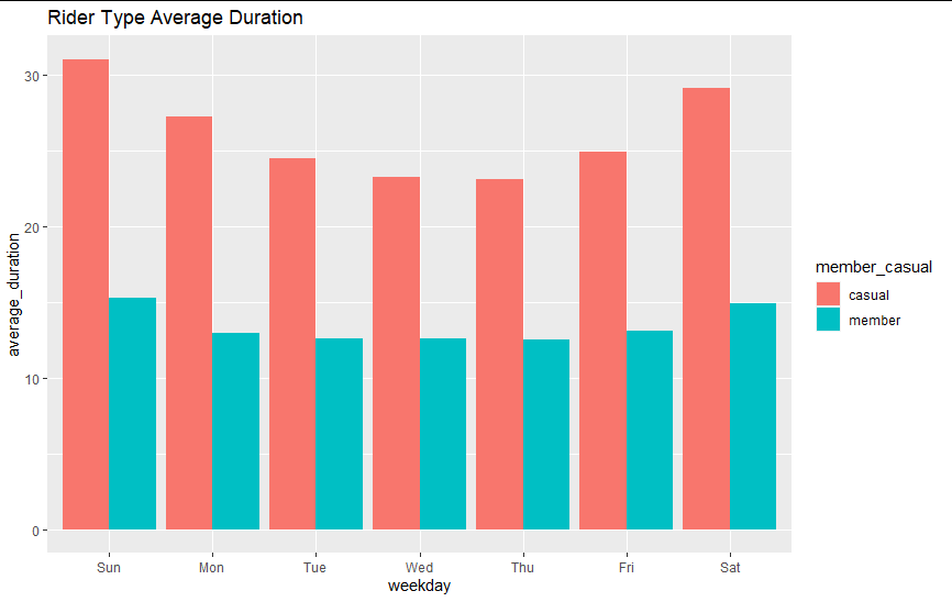
master_trip_2 %>%
mutate(weekday = wday(started_at, label = TRUE)) %>%
group_by(member_casual, weekday) %>%
summarise(number_of_rides = n(), average_duration = mean(ride_length_mins)) %>%
arrange(member_casual, weekday) %>%
ggplot(aes(x = weekday, y = average_duration, fill = member_casual)) +
geom_col(position = "dodge") +
ggtitle("Rider Type Average Duration")
master_trip_2 %>%
mutate(weekday = wday(started_at, label = TRUE)) %>%
group_by(member_casual, weekday) %>%
summarise(number_of_rides = n(), average_duration = mean(ride_length_mins)) %>%
arrange(member_casual, weekday) %>%
ggplot(aes(x = weekday, y = number_of_rides, fill = member_casual)) +
geom_col(position = "dodge") +
ggtitle("Rider Type Number of Bikes")
master_trip_2 %>%
mutate(master_trip_2$rideable_type, label = TRUE) %>%
group_by(rideable_type, member_casual) %>%
arrange(member_casual, rideable_type) %>%
summarise(number_of_rides = n()) %>%
ggplot(aes(x = rideable_type, y = number_of_rides, fill = member_casual)) +
geom_col(position = "dodge") +
ggtitle("Bike Types Usage Difference")
- Saturday and Sunday is always be dominated by casual member, it's twice than the member type users, outside that is dominated by member type user.
- No members are using the docked bike, it's only popular on casual member. But it's still the least popular than the other bike type
- Docked bike is the least popular among the user
- Casual users ride the longest average duration
- The amount of casual members are almost half of the entire user count, it's occupied 40% of the total user population
- The company can make a promotion/marketing strategy focused on Saturday and Sunday for effective and efficient on converting the casual to member user
- Create a duration based promotion milestone and Weekend promotion on the membership program
- Too many missing station name is missing Adding auto completion of station name by comparing it with the langitude and longitude.
- There are 652 of ride length under/equal than 0 minutes Adding validation upon the input should do the job to lessen the data error
- There are 4067 of ride lgnth more/equal than 1 day Giving reminder or limitation of 1 day rent, and then giving an overcharge fee for more than a 1 day rent will lessen the more than 1 day bike rent


