Welcome to your Fall 2022 semester and STA130! STA130 Lectures are Monday's 9:10AM/2:10PM ET for L0101/L0201, and STA130 Tutorials are Friday's 9:10AM/2:10PM ET for L0101/L0201. The Fall 2022 term begins September 8, but we won't meet in person for a tutorial on the first Friday, September 9th; instead, you are expected to use your two-hour tutorial block to review the course website and get a head start on familiarizing yourself with R based on your review of the course website. See you in Lecture on Monday, September 12th!
-- STA130 Instructor Prof. Scott Schwartz
Assistant Professor, Teaching Stream
Director, Data Science Programs for Statistical ScienceP.S. Just call me Scott
Prior to Winter 2020 this was an In-Person course (e.g., F18, F19, W20). From Fall 2020 to Winter 2022 it was transitioned to an Online course (e.g., W22). The current course transitions these iterative course developments back into the previous In-Person format. Specifically, the Winter 2022 Online .ppt and pre-recording material is integrated into leveraged and reworked Rstudio Rmd and beamer pdf materials of the previous In-Person courses.
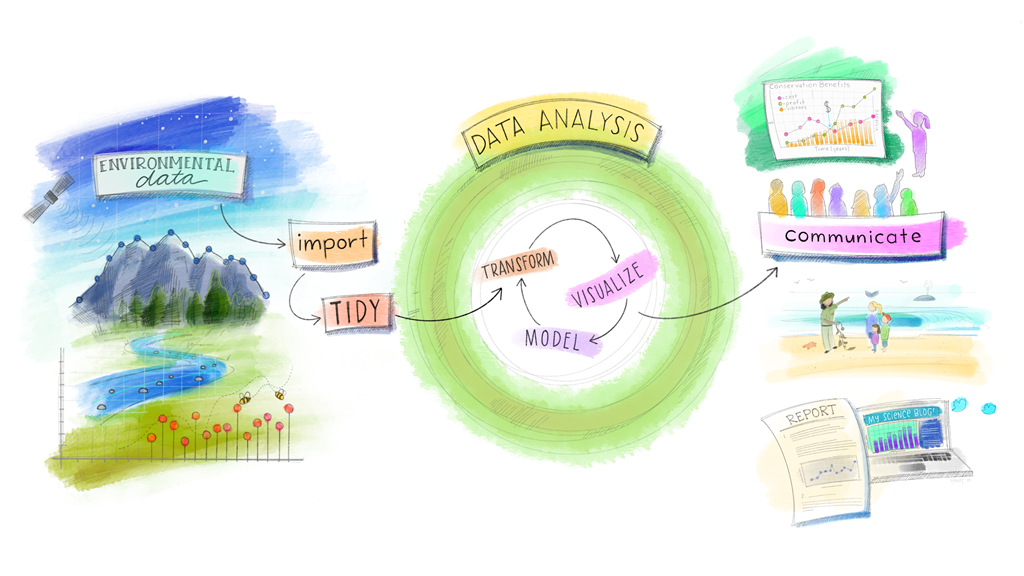
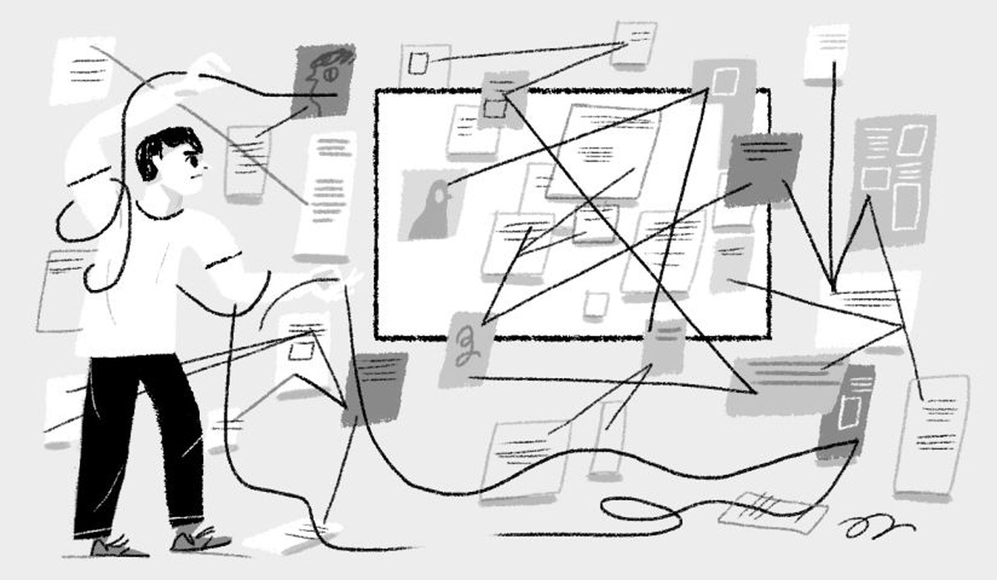
At the highest level, the course activities are meant to develop and practice the final two steps the statistical and data science workflow:
| 1. We'll not be making you struggle to get data yourself 2. Extract meaning from data through coding and analysis 3. Communicate findings through writing and speaking |
 |
|---|---|
| Dr. Julia Lowndes' version of Grolemund & Wickham's classic R4DS schematic illustrated by @Allison_Horst. |
Specifically, STA130 has the following 5 Learning Objectives:
- Implement the computational steps involved in the management and statistical analysis of data using R.
- Carry out a variety of statistical analyses in R and interpret the results of the analyses.
- Clearly communicate the results of statistical analyses to technical and non-technical audiences.
- Identify appropriate uses of statistical methods to answer questions, including their strengths and weaknesses.
- Describe how statistical methods can be used to learn from data, including methods for description, explanation, and prediction.
Please see below for information regarding the following topics:
Fall 2022 semester begins Thursday, September 8th. Friday, September 9th there is no tutorial. The first day of class and the first day of tutorial occur during the week of September 12th.
| Week | Week of | Topic | Monday Lec | Thursday 5PM | Friday Tut | Friday 10PM |
|---|---|---|---|---|---|---|
| 1 | Sep 12 | Jupyterhub, Rstudio, R Basics | 9:10AM/2:10PM | HW1 Due | 9:10AM/2:10PM | Tut 1 Due |
| 2 | Sep 19 | Distributions and Statistics | 9:10AM/2:10PM | HW2 Due | 9:10AM/2:10PM | Tut 2 Due |
| 3 | Sep 26 | Data Wrangling with Tidy | 9:10AM/2:10PM | HW3 Due | 9:10AM/2:10PM | Tut 3 Due |
| 4 | Oct 3 | One/Two Sample Hypothesis Testing | 9:10AM/2:10PM | HW45Part2 Due | 9:10AM/2:10PM | Tut 4 Due |
| 5 | Oct 10 | *THANKSGIVING DAY: NO CLASS, RESCHEDULED | HW45Part3 Due | 9:10AM/2:10PM | Project Introduction | |
| 6 | Oct 17 | Bootstrap Confidence Intervals | 9:10AM/2:10PM | HW6 Due | 9:10AM/2:10PM | Tut 5 Due |
| 7 | Oct 24 | Midterm Review | 9:10AM/2:10PM | 9:10AM/2:10PM | Midterm Exam | |
| 8 | Oct 31 | Simple Linear Regression | 9:10AM/2:10PM | HW7 Due | 9:10AM/2:10PM | Tut 6 Due |
| 9 | Nov 7 | READING WEEK | ||||
| 10 | Nov 14 | Multivariate Linear Regression | 9:10AM/2:10PM | HW8 Due | 9:10AM/2:10PM | Tut 7 Due |
| 11 | Nov 21 | Classification Decision Trees | 9:10AM/2:10PM | HW9 Due | 9:10AM/2:10PM | Tut 8 Due |
| 12 | Nov 28 | Ethics, Confounding, and Study Design | 9:10AM/2:10PM | HW10 Due | 9:10AM/2:10PM | Tut 9 Due |
| 13 | Dec 5 | Final Review | 9:10AM/2:10PM | |||
| *Oct 10 -> Dec 8th Reschedule | Thursday | |||||
| Dec 8th | ||||||
| 9:10AM/2:10PM | ||||||
| Project (DUE) | ||||||
| Presentations |
Ivan and Rahul Selvakumar have put together some resources for helping you get better at R (found through the Department along with some YouTube channels and MOOCs). These specific resources are highlighted in where appropriate in the outline below as well.
https://mdl.library.utoronto.ca/support/workshops-and-training
R self-paced introduction from the Department Of Statistical Sciences
- Students can use the code and modules provided to gain some hands-on-experience with R. It covers most of the stuff that students do in STA130 and some more (Using github, maps and etc ) which can be helpful for Statistics competitions and Kaggle competitions.
R for Data science (Courtesy of Cindy 😊)
- A thorough book on how R (and its countless packages) can be used to perform data analysis. Although the book delves into a lot of complicated ideas it can be a great place for those who want to venture outside of STA130.
Another excellent book that focuses more on R markdown which is an excellent resource for students who want to learn how to create dynamic pdfs, html files or word documents with R. Having a good understanding of this can be a plus for resume
- A more handhold-y youtube guide that involves the basic codes aspects of R. I think this is great for students who are finding it difficult to execute even a single line of code in R. (just to be clear this is just for this video and not the course that they are running which is way too expensive)
RStudio’s own education guidelines
This covers a few basic ways students (and others) can get started with R. The main page includes a few videos, tutorials, books, and a flowchart with how to get started with R. I also recommend going through until the Intermediate stage which covers, design elements such as visualisation, cheatsheets, statistical models such as regression, and some interactive applications (although this tends to be a more advanced)
- This is just a workshop held by UofT. Its supposed to be a very basic introduction to R and Rstudio.
The course project is meant to give you an example of what it can be like to be a statistician doing applied work. To give you an authentic experience, you'll work on data from one of my own current projects, and you'll see what real research work is like (at least for an '
Before I moved to UofT I taught at the University of Virginia School of Data Science. Fun fact: The UVA School of Data Science is the 12th school of the premier US university originally founded by Thomas Jefferson, the principal author of the US Declaration of Independence.
While I was at UVA I met Dr. Heman Shakeri who works in conjuction with the Department of Biomedical Engineering and Systems Biology and Biomedical Data Sciences. Heman's (Dr. Shakeri's) research involves using "data-driven identification and control of high-dimensional dynamical systems" to detect deviations away from normal cellular function and intervene to interrupt the pregression of cancer before it can establish a deleterious cellular homeostasis. As with many people, Heman's interest in this area is motivated by the personal experience of a close family friend. Heman's work is movtivated by his hope that his research will help give family's more time with their loved ones and close friends.
In my career I've worked in Integrative Biology, Nutrition and Complex Disease, and Next Generation Sequencing labs. I've actually been a "Bioinformatician" for about the same amount of time that I've been a "Data Scientist" (in industry) and "Statistician" (here in academia). So, with that in mind, when Heman and I talk about our research, the conversation looks something like this:
The data we will work with is based on advances in the fields of Flow Cytometry for single cell analysis and Mass Spectrometry for measurement of cellular proteomic processes (the phenotypical process endpoint of cellular function and behavior). Based on these technologies, the multivariate landscape of proteomic activity can be measured for a single cell in any experiemental condition for any cell type at scale (e.g., cellular lines with a cancerous genotype at various stages of progression). By understanding typical cellular homeostatis of healthy and deliterious cells, and observing the phenotypical transformation of cellular proteomic homeostatsis over time in response to different experimental conditions, we may eventually be able to understand how to direct deleterious cellular states to transition into non-deleterious states. And with the ability of "data-driven identification and control of high-dimensional dynamical systems" we'll be able to fight cancer!
Now, if you didn't catch all (or any) of that on your first reading, that's normal. I'm a seasoned professional (I got my PhD in Statistical Science in 2010) and you're a first year college student... I have a 20-year head start on you. The first thing to do here to begin increasing your understanding is to read things several times, slowly and carefully; and, sometimes stopping and pausing to make sense of a word or a concept. While it's not always going to make sense to do this for every part of something you're reading, try it out on the above "sciency" paragraph and see if you can decipher the information there. Once you've done that, and maybe have a better sense of the different scientific pieces of the project, then let's move on to breaking it down with a little more with more focus on the data rather than the science and technology.
The data observations simultaneously measure 22 so-called AP-1 transcription factors and 4 phenotype proteins. So there are 26 total variables, 22 of which are thought of as "casues" and 4 of which are thought of as "outcomes". Each measurement is taken on a single cell; but, we can actually measure lots and lots of individual cells at once; and, we can do the measurements under different experiemental conditions, which lets us repeatedly observe these 22 variables over lots of different cells under lots of different treatment conditions (such as at different treatment conditions at different stages of cancer progression).
- How can we measure the progression over time? Actually, we can't measure the same cells over and over. To make a measurement on a cell we have to destroy it... but, if we take a batch of cells (in a specific experimental condition) then we can split the cells up into groups and make the measurements on the different groups at different times; thus, we observe "the progression of the experimental condition over time".
So the experiment based on condition
$x$ and time$t$ produces the following tidy data table
TF1 TF2 TF3 $\vdots$ TF20 TF21 TF22 Y1 Y2 Y3 Y4 Drug Dosage Time Rep 1 2 $\vdots$ $n$ where the total number of observations
$n = \sum_x \sum_t n_{xt}$ is the sum of all the samples$n_{xt}$ in each condition$x$ and time$t$ (which will be different since different batches of cells so we don't always have the same number of cells).
- Note that the "number of individual cells" is the "number of observations" on which the (26) measurements have been made for each experimental condition
$x$ which is defined by two drugs and their dosage, and each condition is repeated a few times for validation purposes.
Hopefully this makes things a little more comprehensible now. And actually, you've just had your first formal experience as a consultant! How so? Well, in my experience as a statistical, bioinformatic, and data science consultant, the exercise you've just done is exactly how the consulting activity goes. You meet someone, they tell you about their applied problem, and then you would work to learn what the context is and understand what their problem actually is. So if you need, review things here a little bit more, and work to make yourself more comfortable with what this project is all about!
- The great thing about being a consultant in a statistical, bioinformatic, or data science role is how much you get to learn about different application areas. It's an especially great context in which to learn because the people you're learning from are experts in their problem and very knowlegable in their domain of expertise. Stastistics and data science in particular are quite unique fields in this regard, since statistical and data science expertise is applicable in so many different areas. This means the natural directionality is that methods are taken to data, and so statistical and data science roles are naturally involve more learning about new areas than is generally the case in other disciplines.
Continuing with the theme of being a statistical consultant, let's start thinking about this problem from a statistical perspective. What analyses would be helpful for this data? Here is my own thought process about what we could do with this data.
-
Do protein levels in experimental condition
$x$ change over time$t$ ?$\longrightarrow$ Two Sample Hypothesis Testing -
Are protein levels at time
$t$ different between experimental conditions$x_1$ and$x_1$ ?$\longrightarrow$ Two Sample Hypothesis Testing -
At time
$t$ in experimental condition$x$ , what is the relationship between different proteins?$\longrightarrow$ Correlation Estimation -
Can we predict cellular phenotypical outcomes
$(Y)$ values/states from transcription factors (TF)?$\longrightarrow$ Regression/Classification -
At what times
$t$ in experimental conditions$x$ can we do this?$\longrightarrow$ Regression/Classification -
At time
$t$ in experimental condition$x$ , what TF are most predictive of cellular values/states$(Y)$ ?$\longrightarrow$ Regression/Classification - Are there patterns in the patterns? Each above analyses is a result, but what's the analysis of the results themselves?
$\longrightarrow$ meta...
Of the analyses proposed above, we've so far only covered Hypothesis Testing. A good place to both get started on the project as well as familiarize yourself with the data would be to start by doing some Hypothesis Testing on the data. In general, you should use the project to reinforce the topics we're learning by trying them out on the project data. Not only will this be beneficial for your learning, but it will help you avoid a last-minute rush to create your material for the Project Poster Presentations on Thursday, December 8th. For example, Confidence Intervals are the next tool we'll cover in the course. How can we use Confidence Intervals in the context of our course project data, specifically with respect to correlation?
Your Course Project will grade (20% of course grade) will be divided up between an initial logistics planning proposal (2% of course grade), a live poster presentation (8% of course grade), and an offline evaluation of your submitted poster presentation slides (10% of course grade).
Your poster presentation and slides will be evaluated based on your presentation of 3 of the 5 distinct categories of analyses noted above (Hypothesis Testing, Confidence Intervals, Correlation, Regression, Classification) and the use of supporting visualizations and explanation.
The group logistics planning proposal is due my midnight on October 28th, which is the same week as the Midterm Exam.
- The requirement to plan project meeting and work logistics with your group during the week of the Midterm Exam is intended to emphasize scheduling during time when it's particularly relevent; and, to perhaps generate useful opportunties for group study sessions, so hopefully this is something you're doing sooner rather than later. It should not be the case that you're rushing to finish this after the Midterm Exam.
The poster presentations will be on December 8th, and project slides will be due on December 8th as well.
 |
 |
|---|
Outstanding projects will successfully accomplish the required tasks as part of a coherent narrative addressing the bigger picture of the project: what is "good" cellular homeostasis, and how can "bad" cellular homeostasis be changed to be "good"?
For the purposes of the course project, your objective is to answer three questions like those from 1-6 above for our data from our collaborator Dr. Shakeri. Question 7 is not required for the project, but you may be interested in pursuing it anyway if you're attempting to submit an outstanding project. In doing so, you would likely address the following questions:
- How do the observed correlations evolve over time under the different experimental conditions?
- Is this temporal dynamic itself predictive of the eventual state of the downstream cellular phenotypes?
- Are the temporal dynamics different or somehow controlled by the experimental conditions?
By looking at these more advanced "meta" questions, we may be able to understand the inter-dependence of the AP-1 proteins, their driving relationship with downstream cellular phenotypes, and how we may be able intervene along this pathway to induce transformation away from deletarious cellular states. If there are certain correlation structures in the TF proteins that leads to good and bad phenotype outcome states
By understanding typical cellular homeostatis of healthy and deliterious cells, and observing the phenotypical transformation of cellular proteomic homeostatsis over time in response to different experimental conditions, we may eventually be able to understand how to direct deleterious cellular states to transition into non-deleterious states. And with this "data-driven identification and control of high-dimensional dynamical systems" we will be able to fight cancer!
There will be 6 project teams of 4 students per TUT group (perhaps with some groups of 3 depending on course enrollments). Working groups are one of the primary communities we are a part of in life. Take advantage of the opportunity to make connections with your peers! Collaborative work is -- and I cannot stress this enough -- A HUGE part of the being a Statistician or a Data Scientist. So take this opportunity to practice being a good team member. Learn from your peers, meet your peers where they're at and be charitable and generous in your interactions with them, and do your best to be supportive and helpful to your team. You'll need to work as a team to plan your project strategy, divide and assign tasks, and collaboratively improve and refine your work. Be constructive and help synergize your teams potential!
Your first group project assignment (worth 2% of the total 20%, i.e., 2%+18%=20%) is to plan the routine and cadence of your group work and meetings. You will submit a proposal for how you plan to collaborate and work together, as well as a general roadmap of your groups strategy for accomplishing the tasks of the course project. Your proposal must detail how you will systematically explore the data and the applicability and results of applying the methods you're learning to the data.
Your proposal MUST also commit your group to a weekly cadence of project work. This is mandatory and not optional for full marks on this proposal.
Your proposal should address the following questions. When will you meet? How will you meet? How will you communicate outside of meetings? How will you determine which group members do which work? What will you do if a group member is not completing the work they agreed to? What will you do if you can't agree on what work the members of the group will do? What will you do if there are problems with group dynamics? The proposal planning your group logistics is due my midnight on October 28th, which is the same week as the Midterm Exam. Your groups proposal will be evaluated based on the expected effectiveness of the plan, and the contingencies put in place by the proposal that give your group the ability to handle adversity and challenge in a self-sufficient manner.
Submit your group meeting and working logistics proposal (expected to be approximately 100-500 words) here on Quercus. Your submitted document must include the names of each member of your group, and each member of your group must have approved and signed the proposal, and each member of the group must submit this document individually in order to receive a grade for this component. If it has not been possible to contact and engage a group member for the purposes of creating the proposal, document your "reasonable and sufficient" attempt to contact the absent group member as an appendix to your proposal.
There are many things to explore in this data. But remember, the project is scored based on your presentation of 3 of the 5 distinct categories, not the exhaustiveness of your analysis. It is worth spending time on exploratory data analysis (EDA) as it will help you form your initial objectives and guide any advanced work you do beyond the basic project requirements; but, if you find your EDA requiring too much time and effort, then you need to quickly determine how you can reduce the scope of your efforts. You will never be able to do everything you want to with a data set, and you need to be comfortable working efficiently towards clear and achieveable objectives while avoiding "analysis paralysis" -- this is a very important skill for being effective and productive as a statistician or a data scientist.
When you're examining the dependency between the proteins, only examine the different proteins within one particular treatment condition at first. If you're consider comparing analyses across different treatment conditions, it's first to best to confirm that repeated batches (
Rep) are behaving reproducibly. If you are starting to compare different treatment conditions, it's best to start by just comparing two different treatment conditions, and perhaps it makes the most sense to compare the first and last timepoints within a drug since those should show the greatest differentiation.
The data for the course project comes from this article finding that the "AP-1 transcription factor network" (i.e., the relative distributions and dependency relationships of transcription factors) are predictive of "cellular plasticity in melanoma" (i.e., how easily changable the phenotypes are melanoma cell lines), and is available for download here
| Phenotype Indicators | MiTFg | Sox10 | NGFR | AXL | |||
|---|---|---|---|---|---|---|---|
| AP-1 transcription factors | ATF2 | ATF3 | ATF4 | ATF5 | Phospho_ATF1 | Phospho_ATF2 | Phospho_ATF4 |
| ATF6 | JunB | c_Jun | JunD | Phospho_S6 | Phospho_c_Jun | Phospho_Erk1 | |
| NF_kappaB | Fra1 | Fra2 | c_Fos | Ki_67 | Phospho_Fra1 | Phospho_c_Fos | Phospho_p38 |
The cellular phenotypes of melanoma cell can be characterized in terms of the HIGH/LOW balance of the four phenotype indicators MiTFg, NGFR, SOX10, and AXL as follows
| Cellular Phenotype \ Gene | MiTFg | NGFR | SOX10 | AXL |
|---|---|---|---|---|
| Undifferentiated | LOW | LOW | LOW | HIGH |
| Neural crest-like | LOW | HIGH | HIGH | HIGH |
| Transitory | HIGH | HIGH | HIGH | LOW |
| Melanocytic | HIGH | HIGH | LOW | LOW |
where the HIGH/LOW distinctions are determined empirically from the data.
 |
|---|
| Slides [Jupyterhub] + Demo [Jupyterhub] | Problem Set [Jupyterhub] due on Quercus by 5 p.m. ET Thursday |
|---|---|
| PollEV In-Class Questions Round 1, 2, 3, 4, 5 |
Week 1 is concerned with introducing students to R and R libraries (like tidyverse), Rstudio and UofT's Jupyterhub. Our primary reference resources in this task are
- the R for Data Science (R4DS) textbook by Hadley Wickham & Garret Grolemund (previously Hands-On Programming with R)
- specifically the Introductory R and R Markdown material
- online Markdown tutorials, cheetsheats, and resources
- the DoSS Toolkit created by seasoned STA130 Profs. Alexander and Caetano et al.
- RStudio R and R Markdown primers
- and see also RStudio's R Markdown and RStudio cheatsheets
- and free online introductions to R from learning websites like datacamp.
The UofT Jupyterhub is a phenomenal resource; however, it is subject to service outages from time to time (which have in the past coincided with assignment due dates), and it can take a long time to load when there's a lot of simultaneous user demand (if a lot of students in our or another class log in at once). When you cannot use UofT Jupyterhub you must use your own local Rstudio instance.
An extremely valuable skill in the context of coding for statistics and Data Science is troubleshooting and figuring things out. Resources like the R for Data Science textbook and the the DoSS Toolkit are excellent recources to learn things in a systematic, structured, and organized manner; however, google, stack exchange/overflow, and coding blog posts can be an invaluable resource for finding quick solutions for coding bugs and suggestions for how to complete a desired analyses. Hopefully through this class you will take the opportunity to build your self-sufficiency and coding-resiliance.
 @AllisonHorst @AllisonHorst |
 @AllisonHorst @AllisonHorst |
|---|
| Slides [Jupyterhub] + Demo [Jupyterhub] | Problem Set [Jupyterhub] due on Quercus by 5 p.m. ET Thursday |
|---|---|
| PollEV In-Class Questions Round 1, 2, 3 | Ungraded Optional Quercus Practice Quiz |
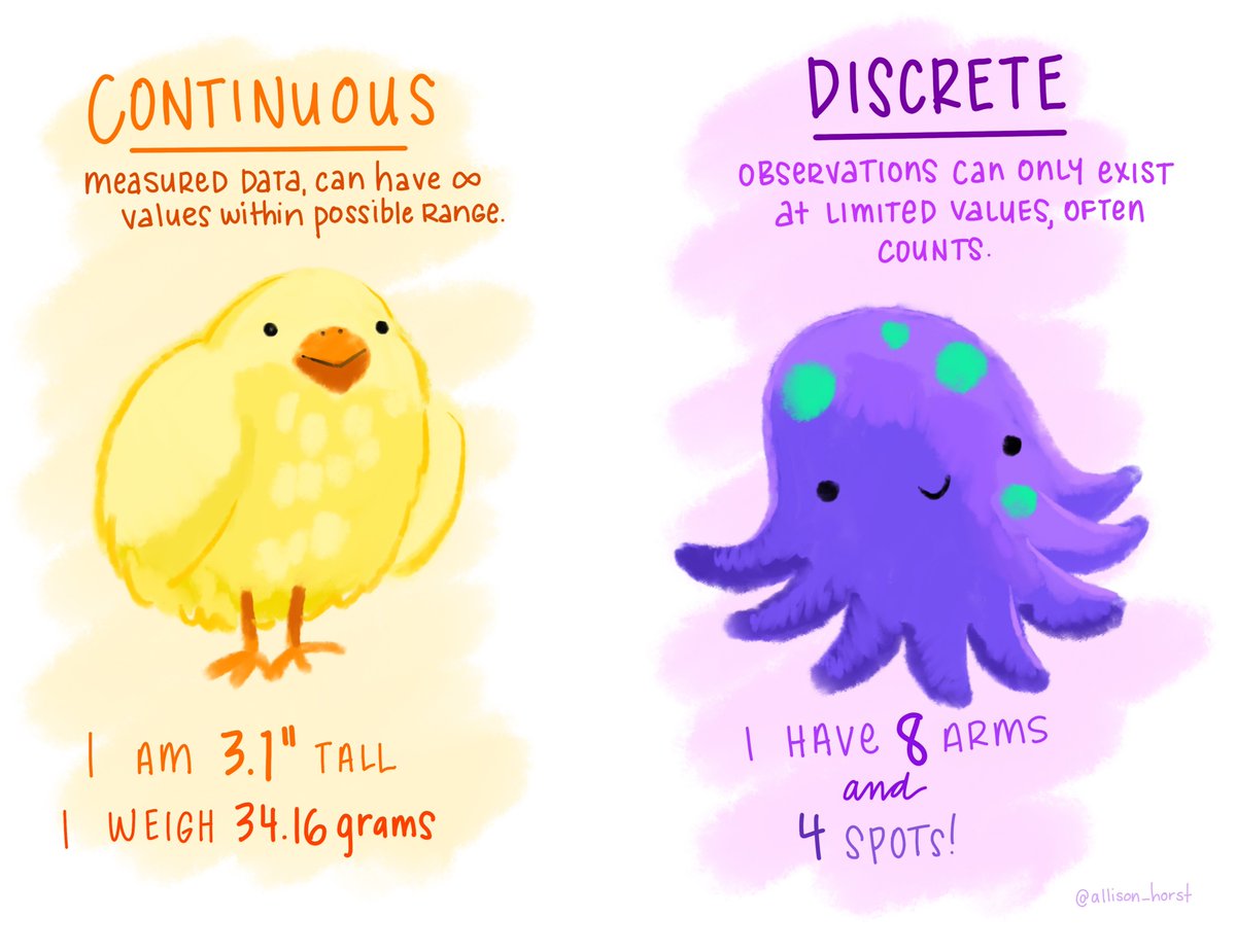
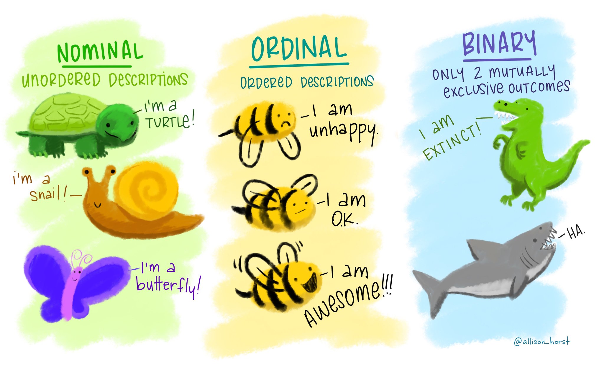
Week 2 differentiates (numerical and ordinal and nominal data types categorical) and explores the technical details of R data types, which directly informs the choice of appropriate visualizations of data. Building on this foundation, the ggplot2 "grammer of graphics" syntax is then introduced (with associated learning and refernce resources listed below) using the examples of bar, histogram, and boxplot geom_'s (but of course there are MANY, MANY other kinds of plots, too). The fig.size and fig.width R Markdown sizing parameters are also introduced at this stage (and again see below for additional R Markdown learning and reference materials). Standard location (mean, median, mode) and scale (IQR, range, variance, standard deviation) statistics for characterizing distributions are introduced, and higher order distributional characterizations are covered (skewness, etc.)
| ggplot2 Resources and References | Markdown Resources and References |
|---|---|
| Official Cheatsheet | RStudio Markdown Cheatsheet |
| Finding Answers | R4DS Introduction |
| Learning Resources | RStudio Introduction |
| Official Usage | knitr Documentation |
| R4DS Textbook | .Rmd Documentation |
| DoSS Toolkit | Markdown Tutorial |
 |
|---|
| Slides [Jupyterhub] + Demo [Jupyterhub] | Problem Set [Jupyterhub] due on Quercus by 5 p.m. ET Thursday |
|---|---|
| PollEV In-Class Questions Round 1, 2, 3 | Ungraded Optional Quercus Practice Quiz |
Week 3 is concerned with defining "Tidy Data" and introducing the following "Data Wrangling" functions from the dplyr library.
filter() |
mutate() |
mean() |
min() |
& |
select() |
case_when() |
median() |
max() |
| |
rename() |
summarise() |
var() |
quantile() |
! |
arrange() |
group_by() |
sd() |
n() |
%in% |
desc() |
is.na() |
IQR() |
sum() |
rm.na=TRUE |
For additional introductions to these topics see the Tidy Data and Transformation of the R4DS textbook. For additional dplyr resources please see the UofT DoSS Toolkit and the official dplyr cheat sheet. Additional advanced data wrangling tools are available through the dplyr and tidyr tidyverse libraries. For additional tidyr resources please see the official tidyr cheat sheet.
 |
 |
|---|
| Slides [Jupyterhub] + Demo [Jupyterhub] | Problem Set [Jupyterhub] Part 2 and Part 3 due on Quercus |
|---|---|
| Strongly Recommended Ungraded Quercus Practice Quizzes on | respectively at 5 p.m. ET on Thursday this week and next |
| One [Jupyterhub] and Two [Jupyterhub] Sample Hypothesis Tests | Ungraded Optional Quercus Practice Quizzes One and Two |
Week 4 is extremely packed begins an extensive coding assignment, Part 2 of which is due at the original 5 p.m. ET time on Thursday during Week 4, and Part 3 of which is due at 5 p.m. ET time on Thursday of Week 5. Both Part 2 and 3 each have one optional question. The remaining parts of the coding assignment are Part 1 which is optional but designed to be more guided and structed to support learning if needed and Part 4 which is optional but Strongly Recommended practice material to test and support your learning.
- There is so much available practice material because there is no lecture during Week 5 after hypothesis testing, and it's important to stay engaged with R and the class so that your progressing and retention provides good support leading into the Week 7 midterm. They hypothesis testing material is potentially quite challenging, and certainly very dense, so the more bolstering and reinforcement of your learning the better.
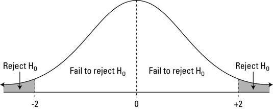
The actual topic of Week 4 is a specific kind of Statistical Inference called Hypothesis Testing. Specifically, we'll examine sample(x, size=n, prop=1/n, replace=FALSE) and for (i in 1:N){ ... }, as well as some cleaver use of group_by(), summarise() and a new diff() function.
- We also introduce
$\LaTeX$ formatting$H_0, H_{1}, H_{A}, \alpha, \bar x, \hat p, \mu,$ and$\sigma$ , which are repsectively$H_0, H_{1}, H_{A}, \alpha, \bar{x}, \hat{p}, \mu$and$\sigma$. This overleaf introduction to formatting math statements in$\LaTeX$ , or the specific topics of subscripts, symbols, and here's a list from stackexchange of some possible accent decorators such as "bar" and "hat".
- If you would find a textbook presentation of these topics helpful, check out sections 2.1, 2.2, 2.3, and 2.4 of Introductory Statistics with Randomization and Simulation from OpenIntro. You can download the textbook for free by using a price of 0, which is absolutely fine since you're students.
- For an additional presentation of two sample permutation-based hypothesis testing, check out the excellent slides from a previous STA130 instructor. These slides are especially recommended for their compelling data examples of "gender bias in promotion recommendation" and "whether or not you can recover from an all-nighter in a couple days".
 |
 |
|---|
- The Course Project will be introduced in Tut on Friday of this week.
- READ the Course Project description BEFORE Tut on Friday of this week.
- There is No Lecture on Thanksgiving (Monday).
- Complete Part 3 of the Week 4 Problem Set [Jupyterhub] due on Quercus by 5 p.m. ET on Thursday.
- It is Strongly Recommended that you complete the Ungraded Quercus Practice Quizzes on One [Jupyterhub] and Two [Jupyterhub] Sample Hypothesis Tests to bolster and reinforce of your learning of the potentially challenging, and certainly very dense, hypothesis testing material.
 |
 |
|---|
| Slides [Jupyterhub] + Demo [Jupyterhub] | Problem Set [Jupyterhub] due on Quercus by 5 p.m. ET Thursday |
|---|---|
| Ungraded Optional Quercus Practice Quiz |
This week introduces a second class of Statistical Inference methods known as Confidence Interval. Specifically, we consider Bootstrapping Confidence Intervals, which are based on the underlying premise of approximating the unavailable population with the available sample (which naturally benefits from increased sample sizes
- The course slides outline the topic list for this section of the course. For another treatment of the Bootstrap Confidence Interval workflow, please see Chapter 13: Estimation from the Inferential Thinking textbook. For more specific explanations of certain topics, or further details of the subtle technical issues, please search out sources online.
 |
|---|
- Monday's lecture period will be will be used as a review for the midterm.
- The Course Midterm will take place in Tut on Friday of this week.
 |
 |
|---|
| Slides [Jupyterhub] + Demo [Jupyterhub] | Problem Set [Jupyterhub] due on Quercus by 5 p.m. ET Thursday |
|---|---|
| Ungraded Optional Quercus Practice Quiz |
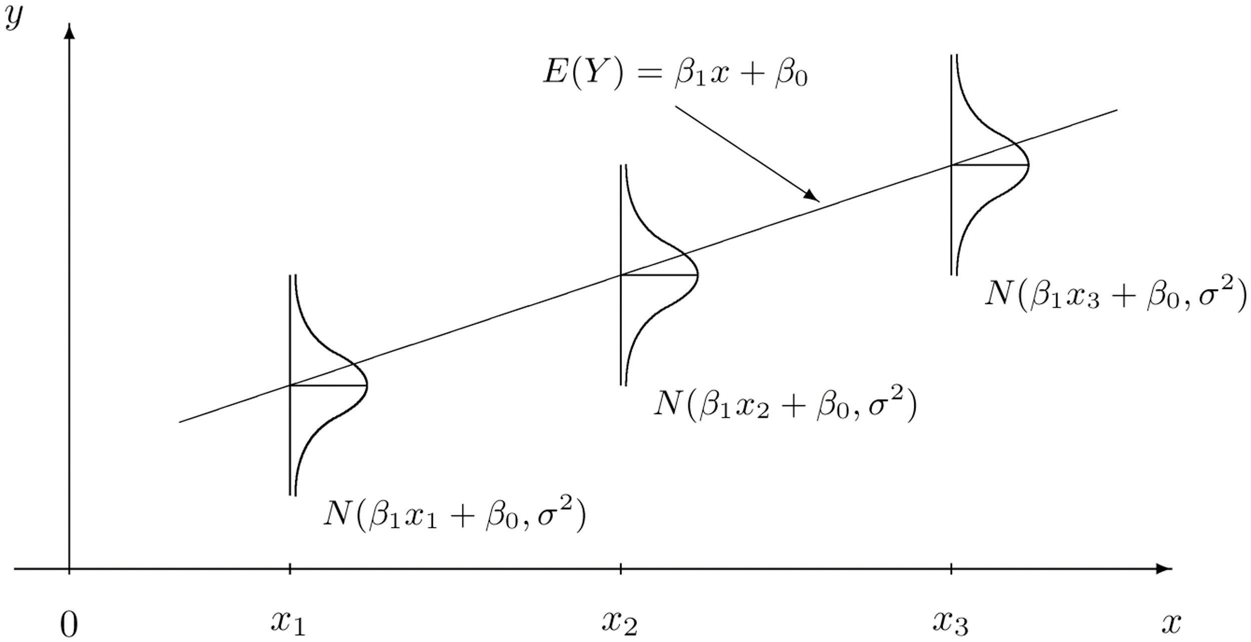
Week 8 introduces the geom_point() plot and facet_grid() layout from ggplot2, as well as the Correlation measure
- As Simple Linear Regression is such a fundamental methodology, if you're looking for further explanations and information you will be able to readily find resources online with some searching.
 |
|---|
Have great break!
 |
 |
|---|
| Slides [Jupyterhub] + Demo [Jupyterhub] | Problem Set [Jupyterhub] due on Quercus by 5 p.m. ET Thursday |
|---|---|
| Ungraded Optional Quercus Practice Quiz + More Practice Questions |
Week 10 extends to the Simple Linear Regression framework into Multivariate Linear Regression. The Prediction exercise is compared to the Hypothesis Testing and Estimation frameworks as another form of Statistical Inference. The Coefficient of Determination
- As Multivariate Linear Regression is such a fundamental methodology, if you're looking for further explanations and information you will be able to readily find resources online with some searching.
 |
 |
|---|
| Slides [Jupyterhub] + Demo [Jupyterhub] | Problem Set [Jupyterhub] due on Quercus by 5 p.m. ET Thursday |
|---|---|
| Ungraded Optional Quercus Practice Quiz |
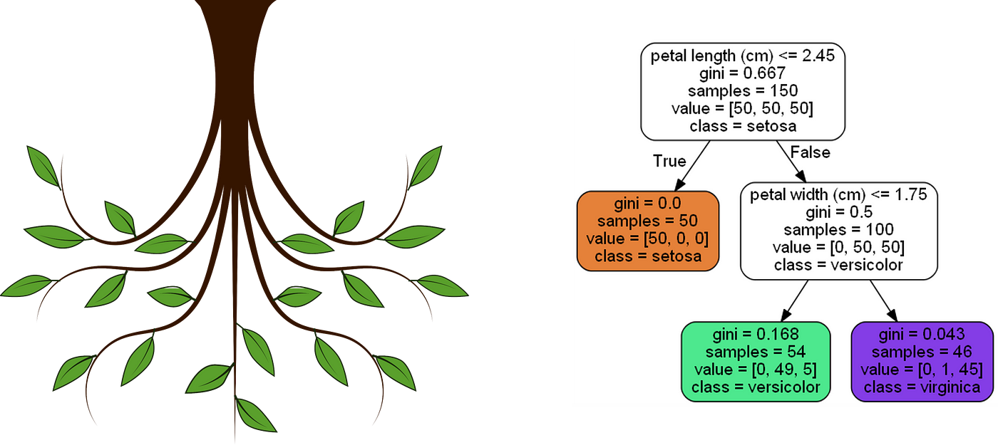
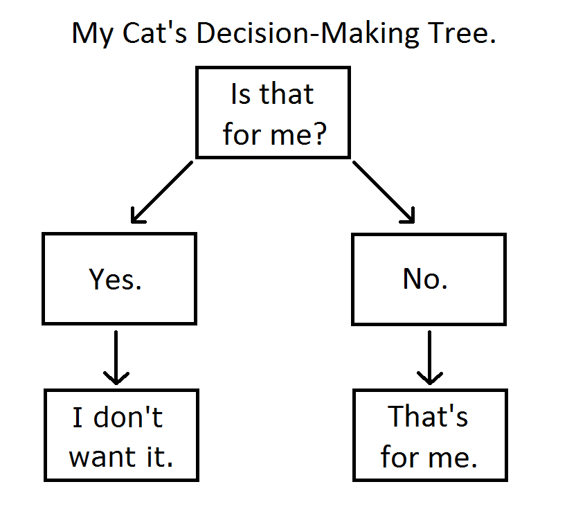
Week 11 introduces Binary (and Multi-Class) Classification Decision Trees. Classifification is a prediction methodology that is related to Regression based prediction and along with Regression completes the prediction category of Statistical Inference. While the Hypothesis Testing and Estimation categories of Statistical Inference are traditionally "statistical", the prediction category is often a part of Machine Learning and Data Science. Simple Linear and Multivariate Regression are examples of statistical models which are used for prediction; whereas, Decision Trees are examples of predictive Machine Learning algorithms which are used for prediction. There are many examples of predictive Machine Learning algorithms which do prediction (such as Random Forests); and, there are statistical models which do clssification (such as logistic regression, which is slightly misnomered).
The difference between Classification and Regression is that Classification predicts "classes" (like "yes" or "no") while Regression predicts real-valued outputs (such as the price of something). When predicting specific classes you are making decisions which are "right" or "wrong" (as opposed to in regression where your prediction is off by some amount called the "residual"). In this sense, Classification is conceptually similar to Hypothesis testing in that Type I and Type II errors characterize the types of incorrect decisions you can make about a hypothesis, whereas in Classification the analogous notions are called False Positives and False Negatives. Based on these error, and the correct classifications called True Positives and True Negatives, a number of "Metrics" are used to quantify the performance of the classification method; namely, for example, precision, sensitivity/recall (True Positive Rate, or one minus False Positive Rate), and Specificity (True Negative Rate, or one minus False Negative Rate). The implications of all of these aspects in the context of a specific application is explored carefully, in addition to their technical specifications. In particular, Confusion Matrices relative to which all these metrics and considerations can be framed are of central importance and are thus a focal point of the discussion and analysis.
As noted, Decision Trees comprise a particular class of Classification Algorithms. The various aspects of Decision Tree methods are explored and detailed, including: node and branching structures, their recursive partitioning treatment of the data, and the thresholding mechanism by which they can favor reducing False Positives or False Negatives (depending on prioritization of these errors implied by the application domain). Model comparision is considered, and the 80/20 Train-Test methodology is reviewed and again applied in the service of this objective.
- As Classification, Confusion Matrices, and Decision Trees (and all related details and terminologies) are such fundamental methodologies in Prediction, Data Science, and Machine Learning, if you're looking for further explanations and information you will be able to readily find resources online with some searching.
 |
 |
 |
|---|
| Slides [Jupyterhub] | Problem Set [Jupyterhub] due on Quercus by 5 p.m. ET Thursday |
|---|---|
| Ungraded Optional Quercus Practice Quiz #1 and (#2)[https://q.utoronto.ca/courses/277998/quizzes/285168] |
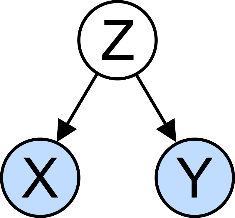
Some fantastic HIGHLY RECOMMENDED reading for this, our last last lecture week of class is the Data Science Ethics chapter from the Baumer et al. Modern Data Science with R textbook. This reading will provide a reflective and structured opportunity to review the key ethics topics that are idiomatic within the data analysis arena. After reviewing these topics ourselves -- including ethics around Webscrapping, APIs, free and informed consent, privacy, and algorithmic bias -- we will then introduce the notion of confounding, through which we will discuss the various forms of experimental and observational study designs; namely, controlled randomized experiements, and prospective, cohort, case-control, and longitudinal studies. If the topics learning about the world through data collection studies interests you then you should seriously consider taking STA304: Surveys, Sampling and Observational Data at some point in your future careers.
- Thursday, December 8th at the usual Monday Lecture time