To successfully compile this code, you need to have Qt installed on your system. A simple option is to download the Qt Creator IDE.
So what is this project all about? If you'd like a dive into some physical background, here we go. Let's assume we want to know which path a classical particle with conserved energy takes between a fixed beginning and ending point. It turns out that, among all paths that the particle could take between the two points, the one prescribed by classical mechanics is the one for which the abbreviated action functional
becomes stationary. This is known as Maupertuis' principle.
In optics, something suspiciously similar is going on. Fermat's principle states that the path that a light ray takes between two points is the one that makes the traversal time stationary. As light moves at an
-th fraction of its vacuum speed given a refractive index
, satisfying Fermat's principle amounts to a stationary optical path length
Here comes the interesting part! We can exploit this correspondence and convert any ray optics problem into one from classical mechanics. Take the following setting: say we assign a refractive index to any point in space. This distribution could model some type of lens, a boundary between two optical media, or anything else we're curious about. At some point we place a light source that emits rays into multiple directions. Now let's forget about optics altogether. Fix some arbitrary, but constant energy value and construct a mechanical potential out of
by the prescription
Next, let a number of particles (all with equal energy and mass
) leave the source location in different directions and find their trajectories in the potential by numerically integrating Newton's second law.
Because of the way we constructed out of
, these trajectories do not only satisfy Maupertuis' principle in their potential, but also Fermat's principle in the refractive index distribution that defined our original problem. The particles move precisely along the light rays that we want to trace! If I got you curious about the analogy between optics and mechanics and if you'd like to learn something about the underlying connection to wave propagation and Huygens' principle, you might also want to take a look into chapter 9 of V.I. Arnold's legendary book 'Mathematical Methods of Classical Mechanics'.
While everything so far is already good to know in theory, I thought it might be even better to have something interactive to play around with. This is why I wrote this (still very preliminary) program which is two things in one: a Newtonian particle and light ray simulation, as these are just two physical perspectives on the same mathematical problem. After entering a function for the refractive index distribution, you can either take the viewpoint of simulating light rays in this distribution, or you can switch to a program mode that displays the derived potential, in which the same plotted rays take the meaning of particle trajectories. Let's see how this works out in practice.
After running the code, you will first see an empty black color map and need to enter a refractive index distribution into the text field on top. For inspiration, here are some toy examples to start with.
After entering
2-1/(1+exp(-7*(sqrt((0.5*x)^2+(0.5*y)^2)-1)))
hitting Animate and letting the animation run through, the plot will look like this:
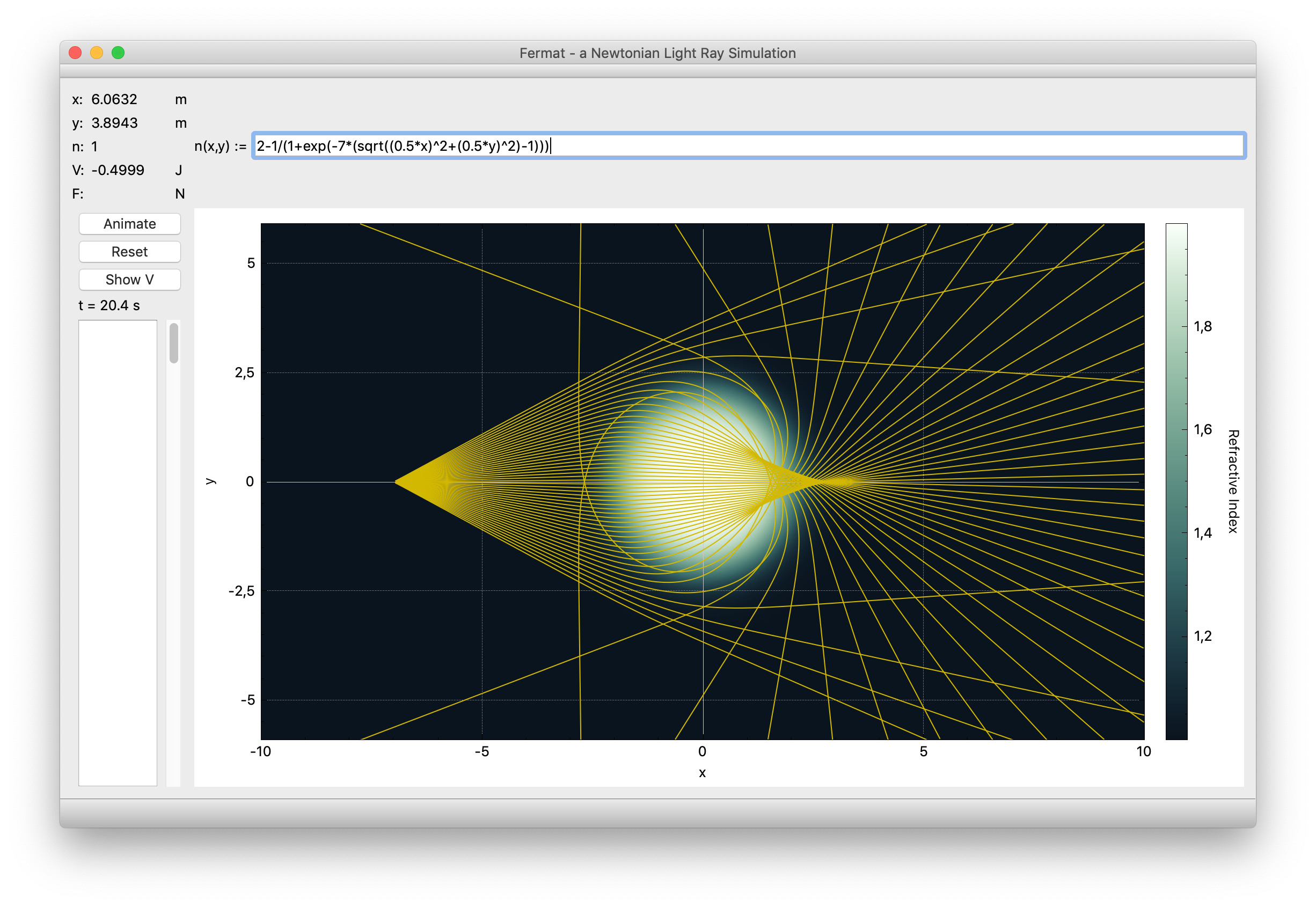 The function may look a bit messy, but think about it like this: plugging the (shifted) radius into a Heaviside step function would give us a precisely disk-shaped distribution around the origin. Replacing the step by a sigmoid function washes out the disk around its boundary.
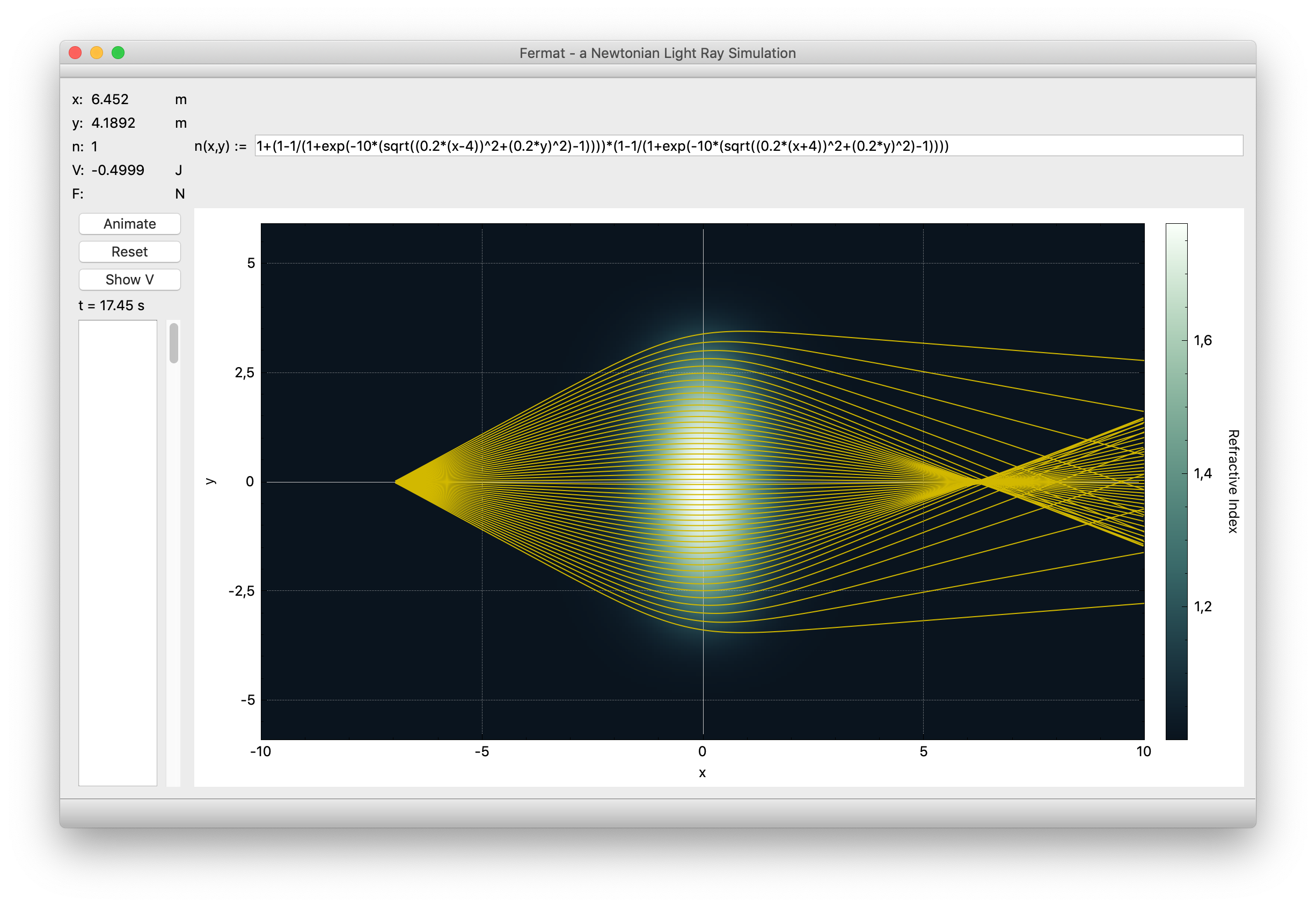
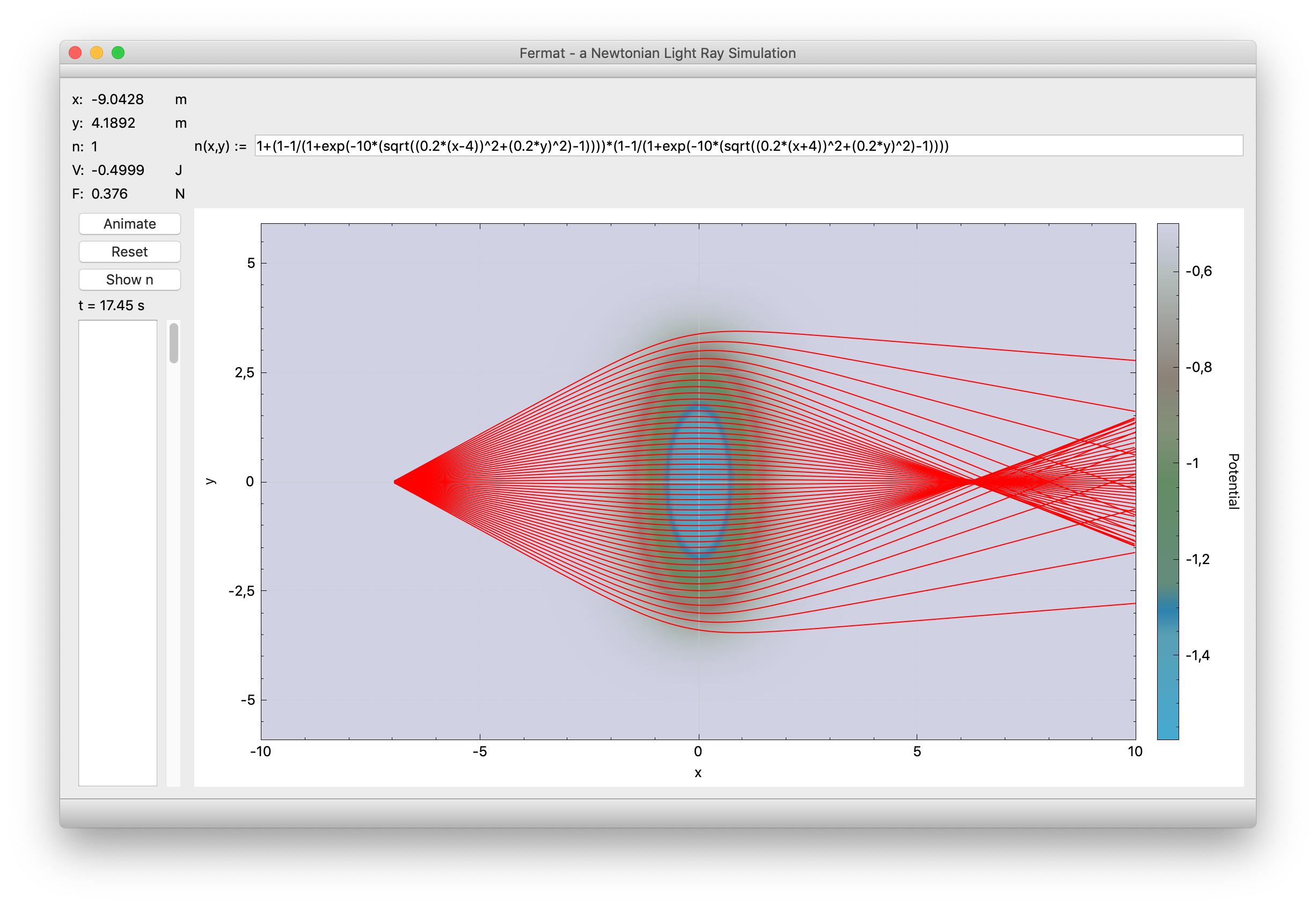
Intersecting (i.e., multiplying the functions of) two eccentrically shifted spheres gets us a biconvex lens. Entering the function
1+(1-1/(1+exp(-10*(sqrt((0.2*(x-4))^2+(0.2*y)^2)-1))))*(1-1/(1+exp(-10*(sqrt((0.2*(x+4))^2+(0.2*y)^2)-1))))
creates a plot that looks like
this:
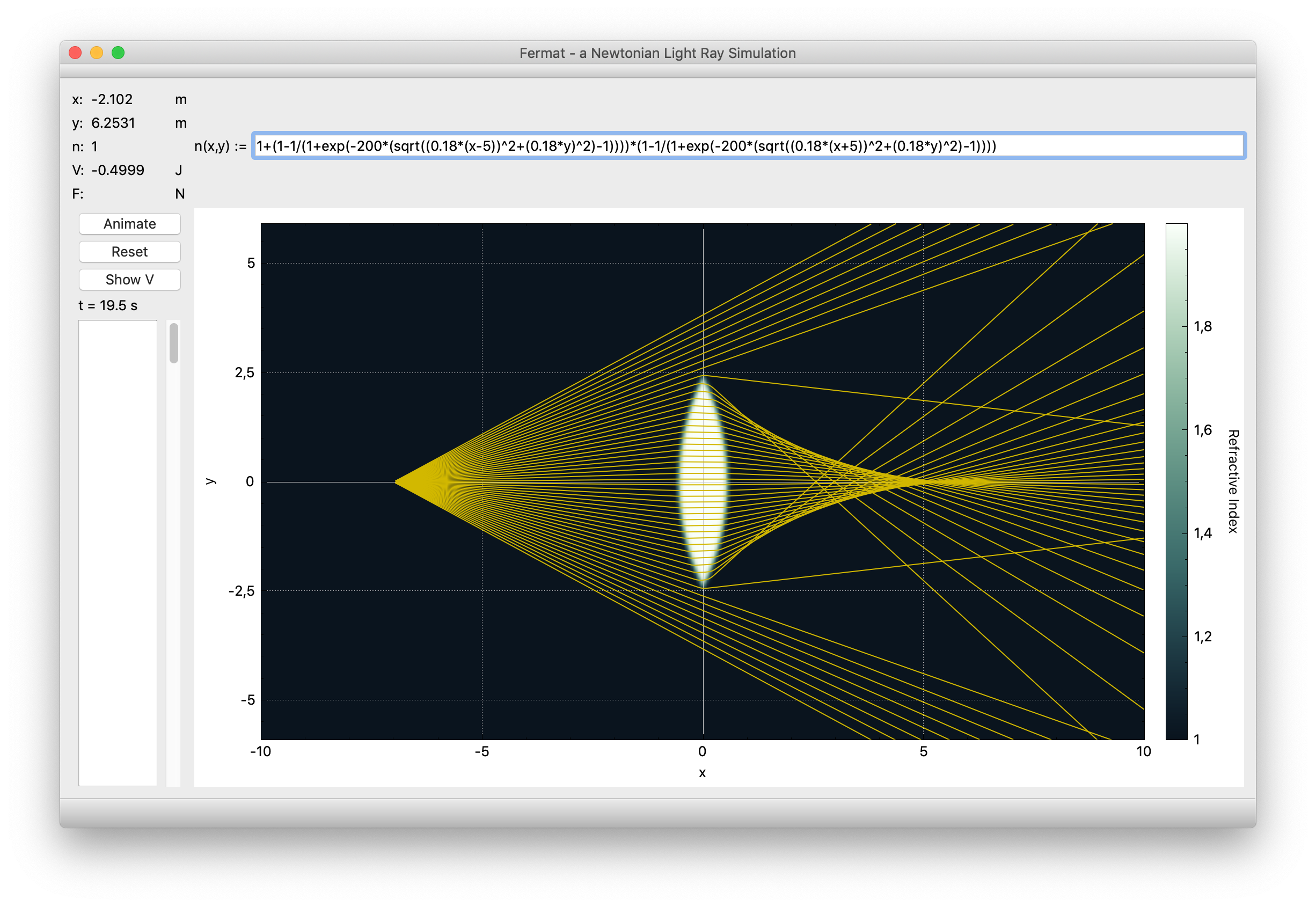
By tweaking the parameters of the function like in
1+(1-1/(1+exp(-200*(sqrt((0.18*(x-5))^2+(0.18*y)^2)-1))))*(1-1/(1+exp(-200*(sqrt((0.18*(x+5))^2+(0.18*y)^2)-1))))
we can also make the lens boundary a lot sharper, getting us
this plot:
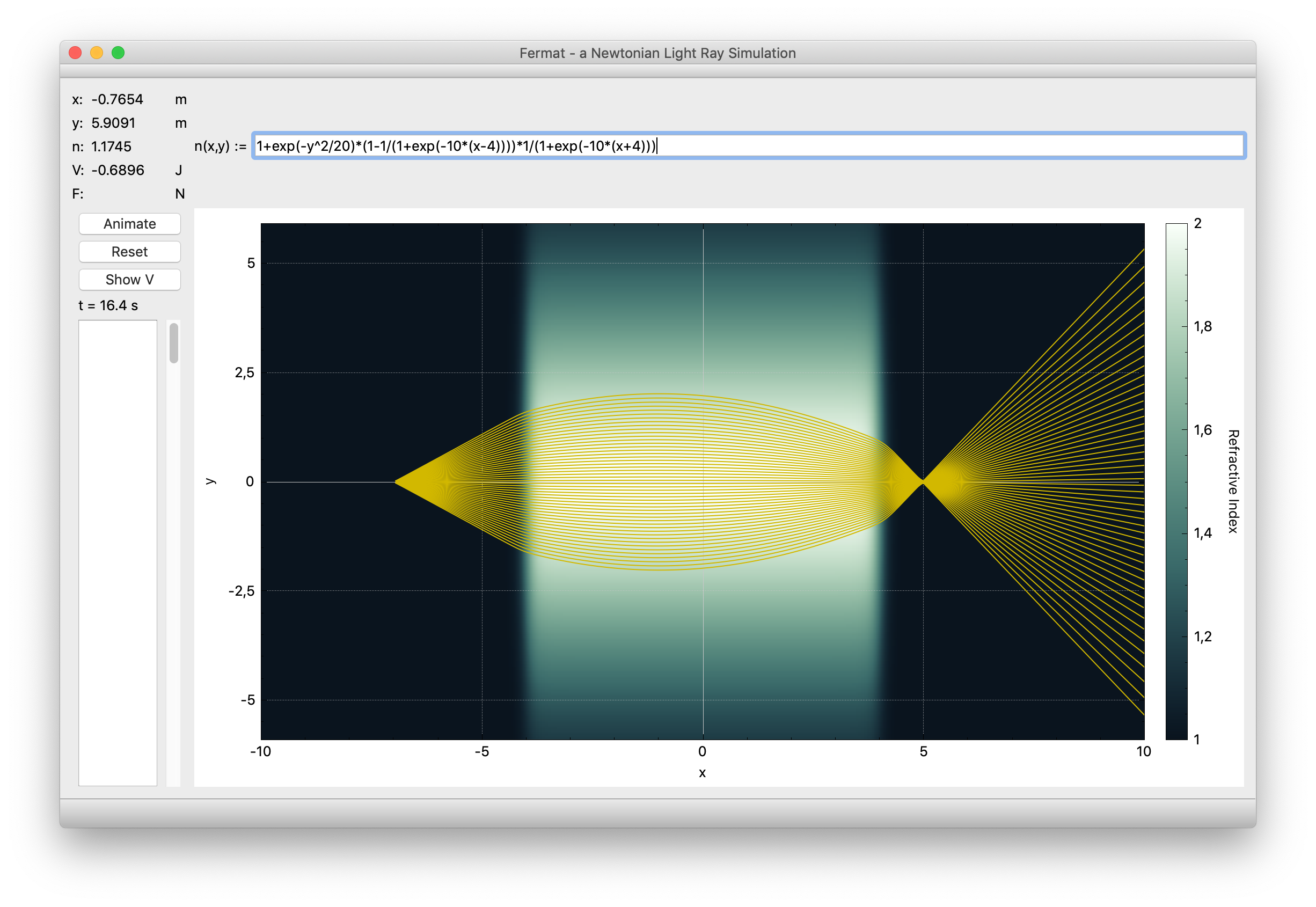
A GRIN (gradient-index) lens achieves its desired effect not by a typical lens geometry, but by an inhomogeneous refractive index distribution of its material. Such a lens can be modeled by the function
1+exp(-y^2/20)*(1-1/(1+exp(-10*(x-4))))*1/(1+exp(-10*(x+4)))
and the plot will look like
this:
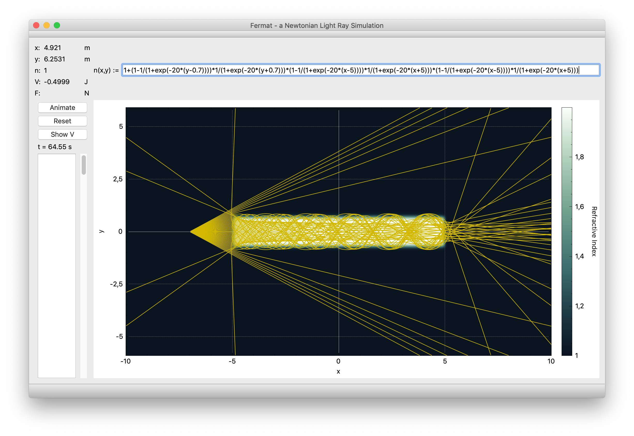
Finally, we can also look at a setup that is modeled after an optical fiber by entering
1+(1-1/(1+exp(-20*(y-0.7))))*1/(1+exp(-20*(y+0.7)))*(1-1/(1+exp(-20*(x-5))))*1/(1+exp(-20*(x+5)))*(1-1/(1+exp(-20*(x-5))))*1/(1+exp(-20*(x+5)))
which gets us
this plot:
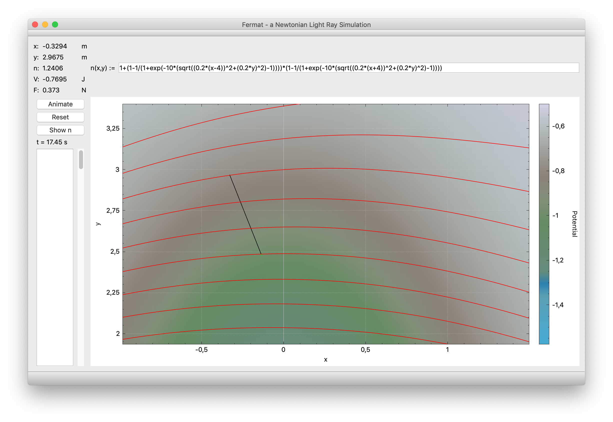
Clicking Show V puts the program into a different mode. The color map now indicates not the refractive index but its corresponding potential (alluding to a height map in geographic color scheme). The rays now have the interpretation of particle trajectories in the potential.
An example plot in potential mode:
In potential mode, right-clicking will draw an arrow indicating the force acting on a particle at the cursor position (left-clicking anywhere will erase it). Zooming in and sampling force arrows along a trajectory allows to easily see why it follows its given path.
A zoomed-in view with a force arrow: