Cosmo-Ages Sequence Calculator (CASC)

A simple Bayesian approach for a set of gaussian ages in a sequence.

Ángel Rodés, SUERC 2020
www.angelrodes.com

How it works

• Install MATLAB or Octave on your computer.
• Download the files CASC.m and BFG.m to the same folder as your data.csv (e.g. Code>Download ZIP and extract all files).
• Run CASC.m in MATLAB or Octave to compute a sequence of ages for samples listed in data.csv.

Input data

Copy your data in a comma-separated file called data.csv with one header line:

Sample name , age , uncertainty , unit name ,  sequential order

data.csv can be created in Excel and save as .csv. Make sure to use . as decimal separator and , as the delimiter.

Samples from the same unit have the same sequential order, being "1" the oldest unit. In case of a gap in the sequential order (e.g. 1, 2, 4, 5), sequential ages will be calculated also for units with no data.

Avoid spaces and symbols in sample and unit names. For example, use "Moraine-1" instead of "Moraine 1".

Example data from Leger et al. (2021) is provided in the data.csv example file.

Under the hood

Age probabilities for each unit (e.g. each moraine) are calculated as:

P(t|T+>T>T-) ~ P(T|t) * P(t|t<T+) * P(t|t>T-)

Where T+, T and T- are the measured data corresponding to the older, contemporary, and younger units. P(t|t<T+) and P(t|t>T-) are the product of the old-to-young and the young-to-old cumulative sums of older and younger age distributions from other units, scaled between 0 and 1.

All distributions are scaled to fit a total probability of 1 for each unit.

Gaussians are fitted to resulting distributions to produce symmetric ages for the units. (BGF, see https://github.com/angelrodes/CEAA)

Graphical output

Two graphs are generated:

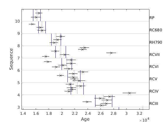
• A scatter + error bar graph with the data (black) and squence ages (blue)

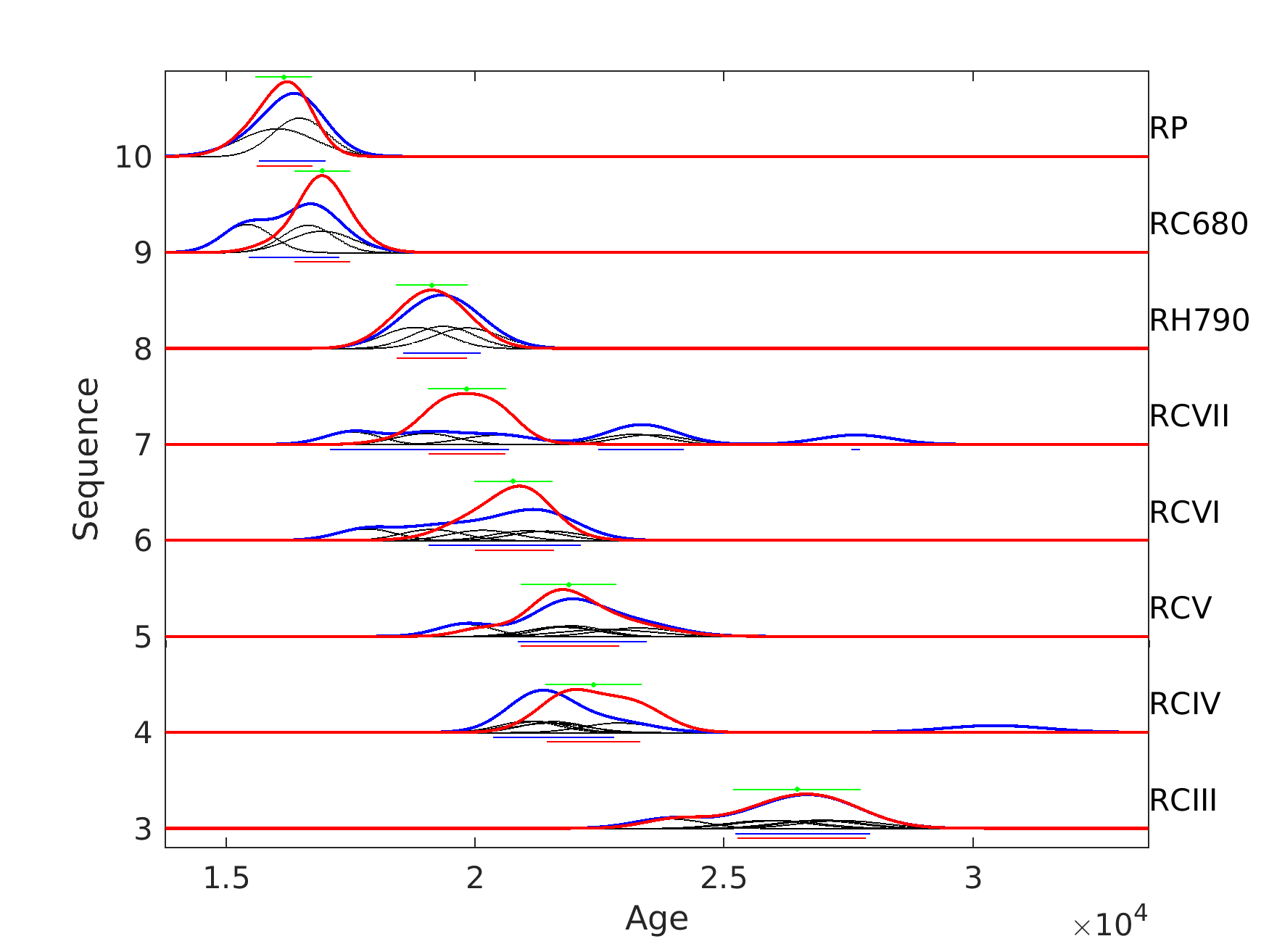
• A plot showing the camelplots corresponding to the original data (individual ages in black and sum of all gaussians in blue), the sequential ages (in red), and Best Gaussian Fits (in green)

References and publications

Part of this code is based on:

• Rodés, Á. (2020). Cosmogenic Exposure Age Averages (CEAA v1.2) [Computer software]. Zenodo.

This code has been used here:

• Leger, T. P. M., Hein, A. S., Bingham, R. G., Rodés, Á., Fabel, D., & Smedley, R. K. (2021). Geomorphology and 10Be chronology of the Last Glacial Maximum and deglaciation in northeastern Patagonia, 43°S-71°W. Quaternary Science Reviews, 272, p. 107194.