
Detecting customers who may commit fraud
- Description
- Data Preprocessing
- Artificial Neural Network
- Statistical Evaluation
- Under Sampling Technique
- Statistical Evaluation of Under Sampling Technique
- Under Sampling Testing on final X_test
- About Author
This project has the objective to help credit card companies detect customers who are potentially committing fraud. The company provides csv data which is data from 280,000 users with 29 independent variables and 1 dependent variable. The desired end result is a model that can classify yes/no between customers who are likely to commit fraud.
- Python
- Artificial Neural Network
- Under Sampling Technique
Feature Engineering is how we use our knowledge in creating new features or simply modifying them while Features Selection is the process of selecting features either combining several features or removing some features. Both methods are intended so that machine learning models can work more accurately in solving problems.
You can download the data here Credit card data
import numpy as np
import pandas as pd
import matplotlib.pyplot as plt
import seaborn as sns

data_ku = pd.read_csv('data_kartu_kredit.csv');
data_ku.shapeStandardizing the Amount Column with the "StadardScaler" method
from sklearn.preprocessing import StandardScaler
data_ku['standar'] = StandardScaler().fit_transform(data_ku['Amount'].values.reshape(-1,1))
standardization is intended to facilitate computation
Removing unused variables.
y = np.array(data_ku.iloc[:,-2])
X = np.array(data_ku.drop(['Time','Amount','Class'], axis=1))
y = dependent variable x = independent variable
To train a model that aims to detect fraudulent users, we use Artificial Neural Network . This method is an adaptive system that can change its structure to solve problems based on external and internal information flowing through the network.l.
from sklearn.model_selection import train_test_split
X_train, X_test, y_train, y_test = train_test_split(X,y,test_size = 0.2 ,
                                                            random_state=111)

X_train, X_validate, y_train, y_validate = train_test_split(X_train,y_train,
                                                            test_size=0.2,
random_state=111)from keras.models import Sequential
from keras.layers import Dense, Dropout
classifier = Sequential()
classifier.add(Dense(units=16, input_dim=29, activation='relu'))
classifier.add(Dense(units=24, activation='relu'))
classifier.add(Dropout(0.25))
classifier.add(Dense(units=20, activation='relu'))
classifier.add(Dense(units=24, activation='relu'))
classifier.add(Dense(units=1, activation='sigmoid'))
classifier.compile(optimizer='adam', loss='binary_crossentropy',
metrics=('accuracy'))
classifier.summary()from keras.utils.vis_utils import plot_model
plot_model(classifier, to_file ='model_ann.png', show_shapes=True,show_layer_names=False)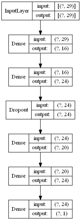
run_model = classifier.fit(X_train, y_train,
                           batch_size = 32,
                           epochs= 5,
                           verbose = 1,
                           validation_data = (X_validate, y_validate))
Epoch 1/5 5697/5697 [] - 9s 2ms/step - loss: 0.0029 - accuracy: 0.9994 - val_loss: 0.0031 - val_accuracy: 0.9994994
Epoch 2/5 5697/5697 [] - 8s 1ms/step - loss: 0.0030 - accuracy: 0.9994 - val_loss: 0.0031 - val_accuracy: 0.9994
Epoch 3/5 5697/5697 [] - 11s 2ms/step - loss: 0.0028 - accuracy: 0.9994 - val_loss: 0.0031 - val_accuracy: 0.9994
Epoch 4/5 5697/5697 [] - 12s 2ms/step - loss: 0.0026 - accuracy: 0.9995 - val_loss: 0.0031 - val_accuracy: 0.9994
Epoch 5/5 5697/5697 [] - 15s 3ms/step - loss: 0.0025 - accuracy: 0.9995 - val_loss: 0.0029 - val_accuracy: 0.9994
plt.plot(run_model.history['accuracy'])
plt.plot(run_model.history['val_accuracy'])
plt.title('model accuracy')
plt.xlabel('accuracy')
plt.ylabel('epoch')
plt.legend(['train','validate'], loc ='upper left')
plt.show()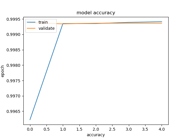
plt.plot(run_model.history['loss'])
plt.plot(run_model.history['val_loss'])
plt.title('model loss')
plt.xlabel('loss')
plt.ylabel('epoch')
plt.legend(['train','validate'], loc ='upper left')
plt.show()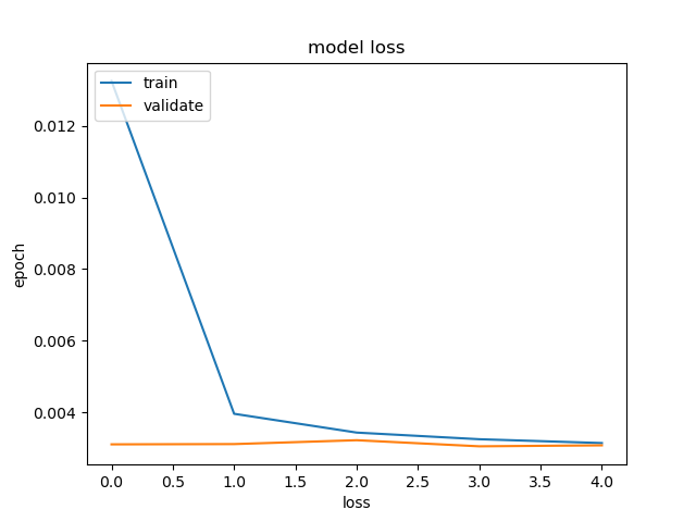
X_test and y_test data y_test is data that has never been seen by the ANN model.
evaluate = classifier.evaluate(X_test,y_test)
print('accuracy:{:.2f}'.format(evaluate[1]*100))
1781/1781 [====== =========================] - 1s 823us/step-loss: 0.0023 - accuracy: 0.9994 accuracy:99.94
prediction_result = classifier.predict_classes(X_test)

from sklearn.metrics import confusion_matrix
cm = confusion_matrix(y_test, prediction_result)
cm_label = pd.DataFrame(cm, columns=np.unique(y_test),index=np.unique(y_test))
cm_label.index.name = 'actual'
cm_label.columns.name = 'prediction'

sns.heatmap(cm_label, annot=True, Cmap='Reds', fmt='g')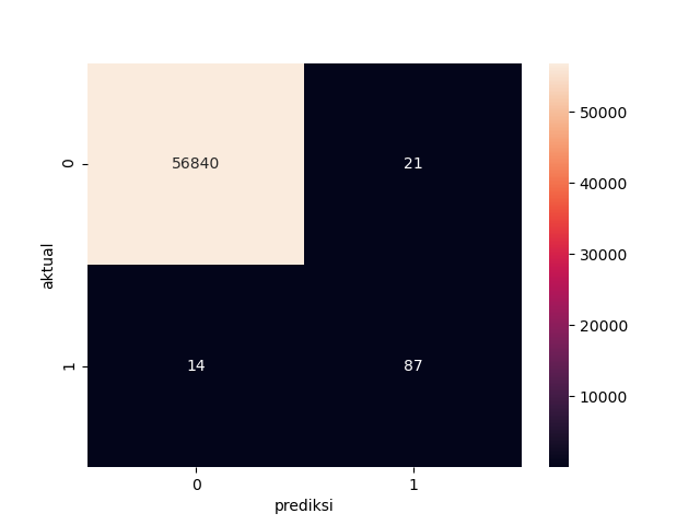
from sklearn.metrics import classification_report
jumlah_kategori = 2
target_names = ['class{}'.format(i) for i in range(jumlah_kategori)]
print(classification_report(y_test, hasil_prediksi,target_names=target_names))
precision recall f1-score support
class0 1.00 1.00 1.00 56861
class1 0.81 0.86 0.83 101
accuracy 1.00 56962
macro avg 0.90 0.93 0.92 56962
weighted avg 1.00 1.00 1.00 56962
At the stage of testing the ANN model on the X_test data and y_test obtained an accuracy of 99.94% which is very high or can be said to be too high so that it is too good to be truth. This accuracy can be explained by looking at the F1-score The f1-score value in class0 has a value of 1, a perfect value that is almost impossible to happen. while for class1 it is at 0.83. So it can be concluded that there is an imbalance dataset which is caused by an imbalance data for those who do cheating and those who do not.
- Undersampling balances the dataset by reducing the size abundant class. This method is used when the amount of data is sufficient. By keeping all samples in the rare class and randomly selecting the same number of samples in the abundant class, a new balanced dataset can be taken for further modeling. In essence, the steps that are different from the initial model are in the data preprocessing process.
index_fraud = np.array(my_data[my_data.Class == 1].index)
n_fraud = len(index_fraud)
index_normal = np.array(my_data[my_data == 0].index) index_data_normal = np.random.choice(index_normal, n_fraud, replace=False )
index_data_baru = np.concatenate([index_fraud, index_data_normal])
data_baru = data_ku.iloc[index_data_baru,:]y_baru = np.array(data_baru.iloc[:,-2])
X_baru = np.array(data_baru.drop(['Time','Amount','Class'], axis=1))X_train2, X_test_final, y_train2, y_test_final = train_test_split(X_new,y_new,
test_size = 0.1,
random_state=111)
X_train2, X_test2, y_train2, y_test2 = train_test_split(X_train2,y_train2,
test_size = 0.1 ,
random_state=111)
X_train2, X_validate2, y_train2, y_validate2 = train_test_split(X_train2,y_train2,
test_size=0.2,
random_state=111)classifier2 = Sequential()
classifier2.add(Dense(units=16, input_dim=29, activation='relu'))
classifier2.add(Dense(units=24, activation='relu'))
classifier2.add(Dropout(0.25))
classifier2.add(Dense(units=20, activation='relu'))
classifier2.add(Dense(units=24, activation='relu'))
classifier2.add(Dense(units=1, activation='sigmoid'))
classifier2.compile(optimizer='adam', loss='binary_crossentropy',
metrics=('accuracy'))
classifier.summary()run_model2 = classifier2.fit(X_train2, y_train2,
batch_size = 8,
epochs= 5,
verbose = 1,
validation_data = (X_validate2, y_validate2))plt.plot(run_model2.history['accuracy'])
plt.plot(run_model2.history['val_accuracy']) plt.title('model accuracy')
plt.xlabel('accuracy')
plt.ylabel('epoch')
plt.legend(['train','validate'], loc ='upper left')
plt.show( )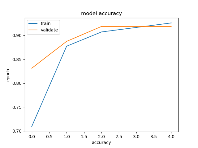
plt.plot(run_model2.history['loss'])
plt.plot(run_model2.history['val_loss'])
plt.title('model loss')
plt.xlabel('loss')
plt.ylabel('epoch')
plt.legend(['train','validate'], loc ='upper left')
plt.show()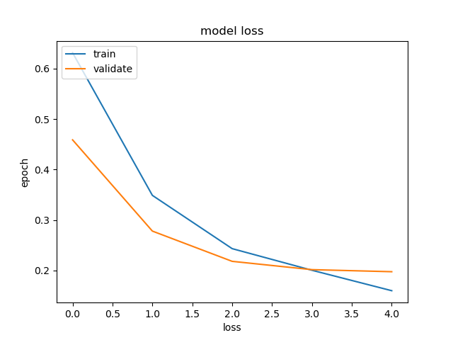
evaluate2 = classifier2.evaluate(X_test2,y_test2)
print('accuracy:{:.2f}'.format(evaluation2[1]*100))
3/3 [============ ==================] - 0s 5ms/step - loss: 0.1846 - accuracy: 0.9213
accuracy:92.13
In the model with the undersampling technique, an accuracy of 92.13% was obtained for a model that had good enough, not too perfect approaching 100%.
hasil_prediksi2 = classifier2.predict_classes(X_test2)

cm2 = confusion_matrix(y_test2,hasil_prediksi2)
cm_label2 = pd.DataFrame(cm2, columns=np.unique(y_test2),index=np.unique( y_test2))
cm_label2.index.name = 'actual'
cm_label2.columns.name = 'prediksi'

sns.heatmap(cm_label2, annot=True, Cmap='Reds', fmt='g')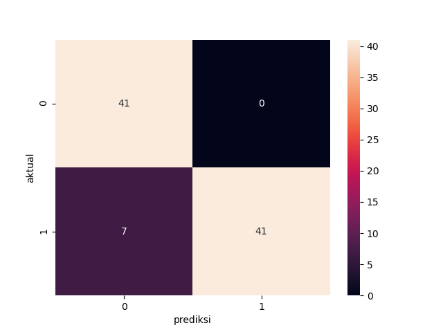
print(classification_report(y_test2, hasil_prediksi2,target_names=target_names)) precision recall f1-score support
class0 0.85 1.00 0.92 41
class1 1.00 0.85 0.92 48
accuracy 0.92 89
macro avg 0.93 0.93 0.92 89
weighted avg 0.93 0.92 0.92 89
This test is running the model on data that has never been seen before. or data that represents the real world.
prediction_result3 = classifier2.predict_classes(X_test_final)
cm3 = confusion_matrix(y_test_final, predicted_results3)
cm_label3 = pd.DataFrame(cm3, columns=np.unique(y_test_final),index=np.unique(y_test_final))
cm_label3.index.name = 'actual'
cm_label3.columns.name = 'prediction'
sns.heatmap(cm_label3, annot=True, Cmap='Reds', fmt='g')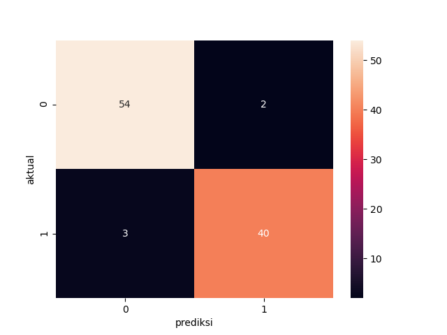
              precision    recall  f1-score   support
      class0       0.95      0.96      0.96        56
      class1       0.95      0.93      0.94        43
    accuracy                           0.95        99
   macro avg       0.95      0.95      0.95        99
weighted avg       0.95      0.95      0.95        99
The test results are quite good although not as high as the initial model, but this model has advantages can be generalized in the sense that it can be applied to real data that is not biased.

Hi, I'm Albara, I'm an industrial engineering student at the Islamic University of Indonesia who is interested in data science field. if you want to contact me you can send a message on the following link.
- Twitter - @albara_bimakasa
- Email - 18522360@students.uii.ac.id