Overview

A robust Python package for automated trend labelling in time series data with a strong financial flavour, implementing SOTA trend labelling algorithms (bibliography) with returns estimation and parameter bayesian optimization capabilities. Main features:

• Two-state (upwards/downwards) and three-state (upwards/neutral/downwards) trend labelling algorithms.
• Returns estimation with transaction costs and holding fees.
• Bayesian parameter optimization to select the optimal labelling (powered by bayesian-optimization).
• Label tuning to transform discrete labels into highly customisable continuous values expressing trend potential.

📜 Table of Contents

• Features
• Installation
• Quick Start
• Core Components
  • A) Trend Labellers
  • B) Returns Estimation
  • C) Parameter Optimization
  • D) Label Tuning
• Usage Examples
• Roadmap
• Contributing
• Bibliography
• License

✨ Features

Trend Labelling Approaches

• Continuous Trend Labelling (CTL):
  • Binary CTL (Up/Down trends) - Based on Wu et al.
  • Ternary CTL (Up/Neutral/Down trends) - Inspired by Dezhkam et al.
• Oracle Labelling
  • Binary Oracle (optimizes for maximum returns) - Based on Kovačević et al.
  • Ternary Oracle (includes neutral state optimization) - Extension of the binary oracle labeller to include a neutral state.

Returns Estimation

• Simple returns calculation
• Transaction costs consideration
• Holding fees support
• Position-specific fee structures

Parameter Optimization

• Bayesian optimization for parameter tuning
• Support for multiple time series optimization
• Customizable acquisition functions
• Empirically tested and customizable parameter bounds

🔧 Installation

pip install tstrends

🚀 Quick Start

from tstrends.trend_labelling import BinaryCTL
from tstrends.returns_estimation import SimpleReturnEstimator
from tstrends.parameter_optimization import Optimizer

# Sample price data
prices = [100.0, 102.0, 105.0, 103.0, 98.0, 97.0, 99.0, 102.0, 104.0]

# 1. Basic naïve CTL Labelling
binary_labeller = BinaryCTL(omega=0.02)
binary_labels = binary_labeller.get_labels(prices)

# 2. Returns Estimation
estimator = SimpleReturnEstimator()
returns = estimator.estimate_return(prices, binary_labels)

# 3. Parameter Optimization
optimizer = Optimizer(
    returns_estimator=SimpleReturnEstimator,
    initial_points=5,
    nb_iter=100
)
optimal_params = optimizer.optimize(BinaryCTL, prices)
print(f"Optimal parameters: {optimal_params['params']}")

# 4. Optimized Labelling
optimal_labeller = BinaryCTL(
    **optimal_params['params']
)
optimal_labels = optimal_labeller.get_labels(prices)

🔩 Core Components

A) Trend Labellers

See the notebook labellers_catalogue.ipynb for a detailed example of the trend labellers.

1. Labellers based on Continuous Trend Labelling (CTL)

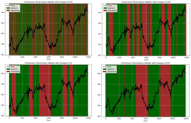
• BinaryCTL: Implements the Wu et al. algorithm for binary trend labelling. When the market rises above a certain proportion parameter omega from the current lowest point or recedes from the current highest point to a certain proportion parameter omega, the two segments are labeled as rising and falling segments, respectively.

  • Parameters:

    • omega: Threshold for trend changes (float). Key to manage the sensitivity of the labeller.
      For instance, for a value of 0.001, 0.005, 0.01, 0.015, the labeller behaves as follows:

    

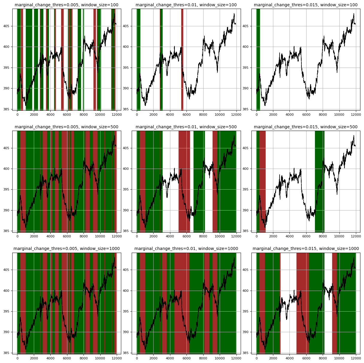
• TernaryCTL: Extends CTL with a neutral state. It introduces a window_size parameter to look for trend confirmation before resetting state to neutral, similar to the second loop in the Dezhkam et al. algorithm.

  • Parameters:

    • marginal_change_thres: Threshold for significant time series movements as a percentage of the current value.
    • window_size: Maximum window to look for trend confirmation before resetting state to neutral.
      For instance, for different combinations of marginal_change_thres and window_size, the labeller behaves as follows:

    

2. Labellers based on the Oracle Labeller

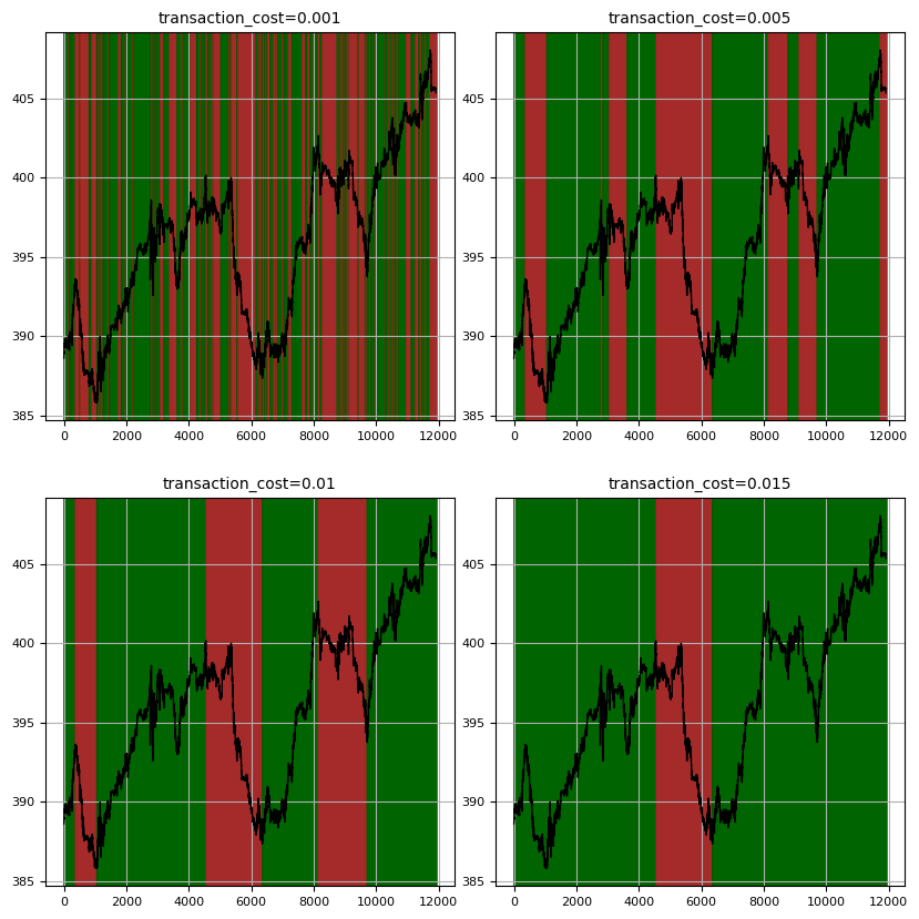
• OracleBinaryTrendLabeller: Implements the Kovačević et al. algorithm for binary trend labelling, optimizing labels for maximum returns given a transaction cost parameter. Algorithm complexity is optimized via dynamic programming.

  • Parameters:

    • transaction_cost: Cost coefficient for position changes.
      For instance, for different values of transaction_cost, the labeller behaves as follows:

    

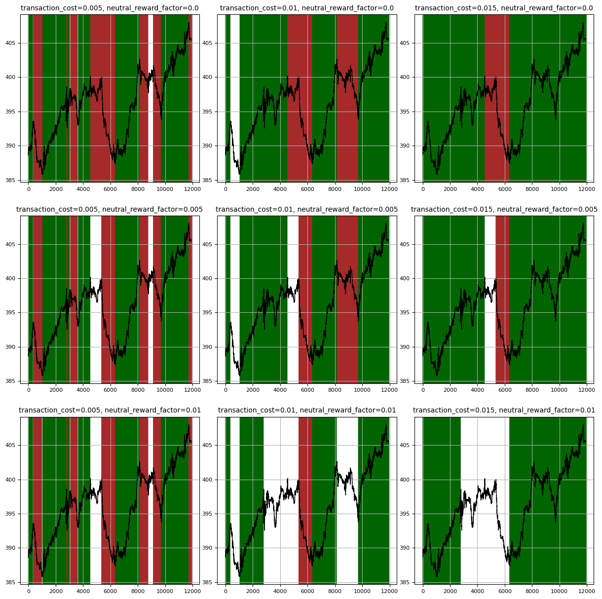
• OracleTernaryTrendLabeller: Extends the binary oracle labeller to include neutral state in optimization. It constrains the switch between upward et downwards trends to go through a neutral state. The reward for staying in a neutral state is managed via a neutral_reward_factor parameter.

  • Parameters:

    • transaction_cost: Cost coefficient for position changes
    • neutral_reward_factor: Coefficient for the reward of staying in a neutral state.
      For instance, for different values of neutral_reward_factor, the labeller behaves as follows:

    

B) Returns Estimation

The package provides flexible returns estimation with transaction costs. It introduces:

• Returns estimation, based on the price fluctuations correctly labelled vs incorrectly labelled.
• Percentage transaction costs, based on the position changes. It pushes the labeller to identify long term trends.
• Constant holding fees, based on the position duration. Useful for ternary labellers to reward the identification of neutral trends.

from tstrends.returns_estimation import ReturnsEstimatorWithFees, FeesConfig

# Configure fees
fees_config = FeesConfig(
    lp_transaction_fees=0.001,  # 0.1% fee for long positions
    sp_transaction_fees=0.001,  # 0.1% fee for short positions
    lp_holding_fees=0.0001,    # 0.0001 constant fee for long positions
    sp_holding_fees=0.0001     # 0.0001 constant fee for short positions
)

# Create estimator with fees
estimator = ReturnsEstimatorWithFees(fees_config)

# Calculate returns with fees
returns = estimator.estimate_return(prices, labels)

C) Parameter Optimization

The package uses Bayesian optimization to find optimal parameters, optimizing the returns for a given fees/no fees configuration. By definition this is a bounded optimization problem, and some default bounds are provided for each labeller implementation:

• BinaryCTL: omega is bounded between 0 and 0.01
• TernaryCTL: marginal_change_thres is bounded between 0.000001 and 0.1, window_size is bounded between 1 and 5000
• OracleBinaryTrendLabeller: transaction_cost is bounded between 0 and 0.01
• OracleTernaryTrendLabeller: transaction_cost is bounded between 0 and 0.01, neutral_reward_factor is bounded between 0 and 0.1

from tstrends.parameter_optimization import Optimizer
from tstrends.returns_estimation import ReturnsEstimatorWithFees
from tstrends.trend_labelling import OracleTernaryTrendLabeller

# Create optimizer
optimizer = Optimizer(
    returns_estimator=ReturnsEstimatorWithFees,
    initial_points=10,
    nb_iter=1000,
    # random_state=42
)

# Custom bounds (optional)
bounds = {
    'transaction_cost': (0.0, 0.01),
    'neutral_reward_factor': (0.0, 0.1)
}

# Optimize parameters
result = optimizer.optimize(
    labeller_class=OracleTernaryTrendLabeller,
    time_series_list=prices,
    bounds=bounds,
    # acquisition_function=my_acquisition_function,
    # verbose=2
)

print(f"Optimal parameters: {result['params']}")
print(f"Maximum return: {result['target']}")

Warning

The acquisition function is set to UpperConfidenceBound(kappa=2) by default. This is a good default choice that balances exploration and exploitation, but you may want to experiment with other values for kappa or other acquisition functions like bayes_opt.acquisition.ExpectedImprovement() or bayes_opt.acquisition.ProbabilityOfImprovement() for your specific use case.

Caution

The default bounds are presetted for relatively constant time series and may not be optimal for all use cases. It is recommended to test the waters by testing the labels with some parameters at different orders of magnitude before optimizing. See optimization example notebook for a detailed example of parameter optimization.

D) Label Tuning (expressing trend potential)

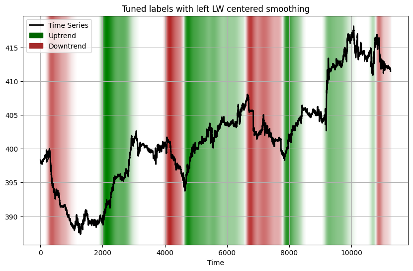
The label tuning module enhances binary and ternary trend labels by adding trend potential information to make them more useful for training prediction models. It transforms discrete labels (-1, 0, 1) into continuous values that express the potential of the trend at each point.

1. Remaining Value Tuner

The RemainingValueTuner transforms labels into continuous values that represent, for each time point, the difference between the current value and the maximum/minimum value reached by the end of the trend. The output values maintain the original label's sign but provide additional information about trend strength:

• For uptrends (1): positive values indicating remaining upside potential
• For downtrends (-1): negative values indicating remaining downside
• For neutral trends (0): values close to zero

This approach is particularly valuable in financial applications where:

• Correctly predicting a trend is most critical at its beginning
• The impact of a prediction depends on the magnitude of the trend's total price change

Key parameters of the tune method:

• enforce_monotonicity: If True, labels in each interval will not reverse on uncaptured countertrends
• normalize_over_interval: If True, the remaining value change will be normalized over each interval
• shift_periods: Number of periods to shift the labels forward (if positive) or backward (if negative)
• smoother: Optional smoother object to smooth the resulting tuned labels (see Smoothing Options below)

from tstrends.label_tuning import RemainingValueTuner
from tstrends.label_tuning.smoothing import LinearWeightedAverage
from tstrends.trend_labelling import OracleTernaryTrendLabeller

# Generate trend labels
labeller = OracleTernaryTrendLabeller(transaction_cost=0.006, neutral_reward_factor=0.03)
labels = labeller.get_labels(prices)

# Create a smoother for enhancing the tuned labels (optional)
smoother = LinearWeightedAverage(window_size=5, direction="left")

# Tune the labels
tuner = RemainingValueTuner()
tuned_labels = tuner.tune(
    time_series=prices,
    labels=labels,
    enforce_monotonicity=True,
    normalize_over_interval=False,
    smoother=smoother
)

2. Smoothing Options

The label tuning module provides smoothing classes to enhance the tuned label output:

• SimpleMovingAverage: Equal-weight smoothing across the window
• LinearWeightedAverage: Higher weights on more recent values (for left-directed smoothing) or central values (for centered smoothing)

Both smoothers support "left" direction (using only past data) or "centered" direction (using both past and future data).

See the label tuner example notebook for a detailed example of label tuning.

🚧 Roadmap

• Transform labels into trend momentum / potential.
• Calculate returns for one subset of labels only.
• Always good to explore more labellers.

🤝 Contributing

Contributions are welcome! Please feel free to submit a Pull Request. For major changes, please open an issue first to discuss what you would like to change.

Please make sure to update tests as appropriate and adhere to the existing coding style.

📚 Bibliography

The algorithms implemented in this package are based or inspired by the following academic papers:

[1]: Wu, D., Wang, X., Su, J., Tang, B., & Wu, S. (2020). A Labeling Method for Financial Time Series Prediction Based on Trends. Entropy, 22(10), 1162. https://doi.org/10.3390/e22101162

[2]: Dezhkam, A., Manzuri, M. T., Aghapour, A., Karimi, A., Rabiee, A., & Shalmani, S. M. (2023). A Bayesian-based classification framework for financial time series trend prediction. The Journal of supercomputing, 79(4), 4622–4659. https://doi.org/10.1007/s11227-022-04834-4

[3]: Kovačević, Tomislav & Merćep, Andro & Begušić, Stjepan & Kostanjcar, Zvonko. (2023). Optimal Trend Labeling in Financial Time Series. IEEE Access. PP. 1-1. 10.1109/ACCESS.2023.3303283.

📄 License

BSD-2-Clause