⚠️ Repository Moved

This repository has been replaced by mosaix-pde.

Please use the new repository for all code, documentation, and issues.

The old code here is preserved for reference only.

pat-pde-opt

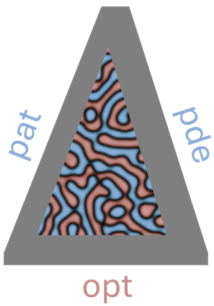
pat-pde-opt is a package for optimizing pattern forming PDEs that appear in different areas of physics, written in JAX. It has code for PDE optimization and control with gradient-based methods and reinforcement learning. We use diffrax for time stepping and implement system-specific solvers, such as semi-implicit Fourier methods and Strang splitting.

You can find the full documentation on read the docs.

Installation

To install the package, we recommend cloning the github repo and then installing locally:

git clone https://github.com/acoh64/pde-opt.git
cd pde-opt
conda create -y -n pde-opt-env python=3.12
conda activate pde-opt-env
pip install -e .

By default, it will install the CPU version of JAX. To use with GPU, run:

pip install -U "jax[cuda12]"

Usage

Here is an example of solving the Cahn-Hilliard equation in 2D with periodic boundary conditions using a semi-implicit Fourier method:

import jax
import jax.numpy as jnp

from pde_opt import PDEModel
from pde_opt import CahnHilliard2DPeriodic
from pde_opt import SemiImplicitFourierSpectral
from pde_opt import Domain
from pde_opt import PeriodicCNN

Nx = Ny = 128
Lx = Ly = 0.01 * Nx

domain = Domain((Nx, Ny), ((-Lx / 2, Lx / 2), (-Ly / 2, Ly / 2)), "dimensionless")

opt_model = PDEModel(equation_type=CahnHilliard2DPeriodic, domain=domain, solver_type=SemiImplicitFourierSpectral)

params = {"kappa": 0.002, "mu": lambda c: jnp.log(c / (1.0 - c)) + 3.0 * (1.0 - 2.0 * c), "D": lambda c: c * (1. - c)}

solver_params = {"A": 0.5}

key = jax.random.PRNGKey(0)
y0 = jnp.clip(0.01 * jax.random.normal(key, (Nx, Ny)) + 0.5, 0.0, 1.0)
ts = jnp.linspace(0.0, 0.02, 100)

sol = opt_model.solve(params, y0, ts, solver_params, dt0=0.000001, max_steps=1000000)

Next, here is an example of using the previous solution as a dataset to fit a neural network for the chemical potential term:

data = {}
data['ys'] = sol
data['ts'] = ts

model = PeriodicCNN(
    in_channels=1,
    hidden_channels=(32, 64, 64),
    out_channels=1,
    kernel_size=3,
    key=jax.random.PRNGKey(0),
)

init_params = {"mu": model}
static_params = {"kappa": 0.002, "D": lambda c: c * (1. - c)}
solver_parameters = {"A": 0.5}
weights = {"mu": None}
lambda_reg = 0.0

inds = [[30,40,50], [50,60,70], [70,80,90]]

res = opt_model.train(data, inds, init_params, static_params, solver_parameters, weights, lambda_reg, method="mse", max_steps=100)

Current Model Implementations

This package is designed to support pattern-forming PDEs across a wide-range of physical systems. We have currently implemented variants of the following equations:

• Cahn-Hilliard equation
  • 2D with periodic boundary conditions
  • 3D with periodic boundary conditions
  • 2D with smoothed boundary method
• Allen-Cahn equation
  • 2D with periodic boundary conditions
  • 2D with constant current conditions + Butler-Volmer kinetics (for battery applications)
  • 2D with smoothed boundary
  • 2D with smoothed boundar and constant current conditions + Butler-Volmer kinetics (for battery applications)
• Gross-Pitaevskii
  • Reduced 2D with periodic boundary conditions
  • Rotating reduced with 2D periodic boundary conditions

TODO

• Arbitrary boundary conditions
• Implicit time stepping
• Multi-GPU support
• Extend to non-Cartesian domains
• WandB logging and checkpointing

License

This code has been published under the MIT licence.