Decoupling Linearizing control for the classic inverted pendulum with MATLAB and Simulink.
A. MODEL OF THE SYSTEM
The process under interest is an inverted pendulum and is described in the following figure.
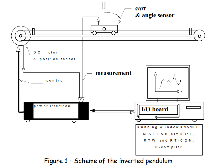
The process consists of a crane driven by a motor, and moving along a guide rail with a length of 1m. On this crane, is placed a pendulum with two rods rotating freely, equipped with weights at their tips. Two incremental encoders allow to know the position of the crane and the angle of the pendulum. Safety stops are located at the end of the way on which the crane is moving.
B. MODELLING OF THE INVERTED PENDULUM
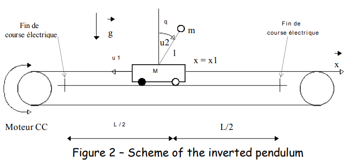
The diagram just below (Figure 2) details the physical parameters of the system. In the sequel, several models will be used, depending on modeling assumptions. Let θ the angle between the pendulum and the vertical, and x the position of the crane. The parameters of the pendulum are the mass of the crane M (=2.4kg), the mass centered at the end of the pendulum m (=0.23kg) and the length of the pendulum L (= 0.36m).
C. PROBLEM STATEMENT
The objective consists in controlling the motion of the inverted pendulum. The controller needs to control the crane position and the angle of the pendulum (for example, one wants to move the carriage bearing the pendulum at a constant angle).
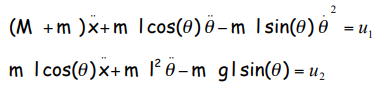
Model 1 : It is assumed that the system has 2 inputs, there is no friction (dry or viscous) and one neglects the inertia of the pendulum. The control inputs are the driving force of the carriage u1 and the torque of the pendulum u2. It should be noted that in the real application, the control input u2 does not exists, and should therefore be considered equal to 0.
The dynamics reads as:
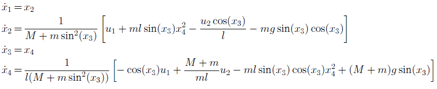
The first model under nonlinear state system (with x1 = x, x2=dx/dt, x3=q, x4=dq/dt.) is defined as:
Setting the I/O linearization as:
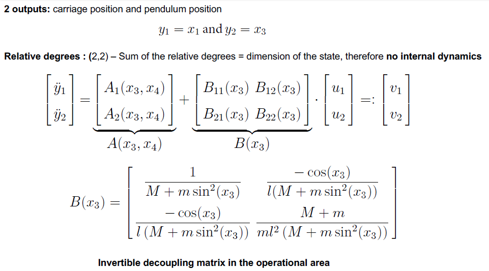 Remark : the control law reads as u = F(x) + G(x) v with v = [v1 v2]T. This control allows pole placement.
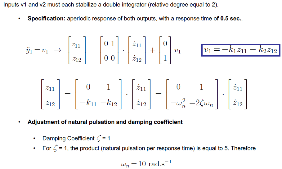
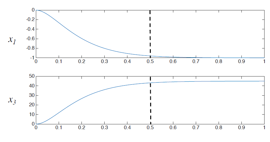
Which logically stabilizes this model 1:
Model 2 : One suppose now that the system has a single input (u2 = 0) , that there is no friction (dry or viscous) and the pendulum inertia is supposed negligible.
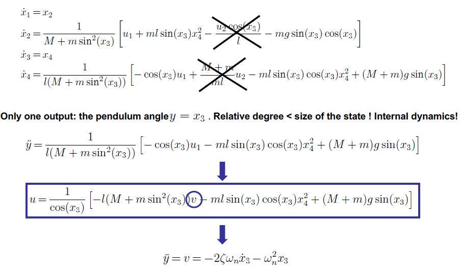
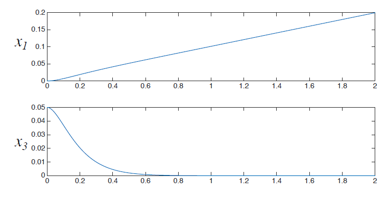
In order to analyze the stability of this model, we will require to check the zero dynamics, which are:
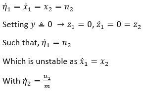
Clearly showing that the state x1 will be "uncontrollably" increasing.
Model 3 : Taking into account the friction and inertia of the pendulum.
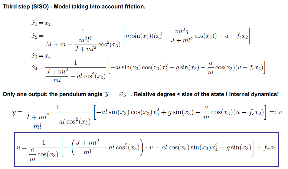
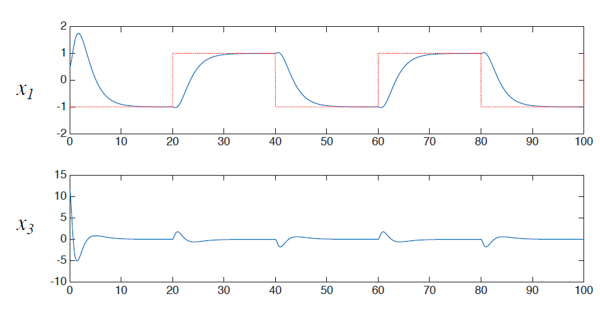
With the aim of design a control law based on a linearizing strategy, allowing to stabilize the both variables, crane position and pendulum angle and tuning the parameters of the controller in order to satisfy the control saturations. Since the "internal" state x1 increase/decrease, according to the sign of x2, "internally", one option would be to add to the pole placement (the last loop) a feedback control for the position, v=...-k1x1:

In this case using x1* and x3* as the reference signal, for a desired position or angle.
Tuning k1 to 0.319 for the model 3, with this "acceptable" behavior:
Model.3.simulation.mp4
Project developed under the M1_EPICO_COSYS Control system class leaded by Frank Plestan at École Centrale de Nantes. All rights reserved to them. For the original formulation of the models check SUJ_PEND_21_22.pdf