aespm -- "A"utomated "E"xperiment on "SPM"

Python interface that enables local and remote control of Scanning Probe Microscope (SPM) with codes.

It offers a modular way to write autonomous workflows ranging from simple routine operations, to advanced automatic scientific discovery based on machine learning.

1. Installation

1-1. Quick installation

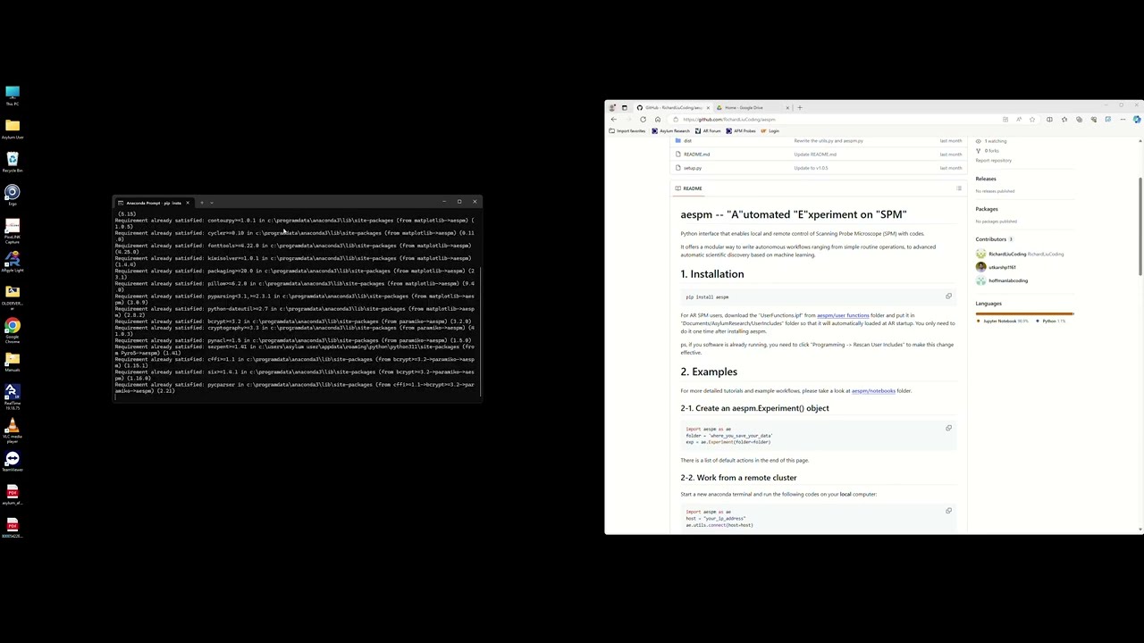
pip install aespm

For AR SPM users, download the "UserFunctions.ipf" from aespm/user functions folder and put it in "Documents/AsylumResearch/UserIncludes" folder so that it will automatically loaded at AR startup. You only need to do it one time after installing aespm.

ps, if you software is already running, you need to click "Programming -> Rescan User Includes" to make this change effective.

1-1-1. Manual Setup of "exe_path"

If your AR/Igor software is not installed in the default path, you need to take the following actions:

1. Install the aespm library as usual.
2. Run the library once (by running import aespm in a terminal or jupyter notebook).
3. Navigate to "Documents-->buffer-->path.txt".
4. Edit the "path.txt" file and paste the path to your "Igor.exe" here.
5. Then it should work now!

1-1-2. Manual Setup of AR versions before v16

If you're using an AR software equal or older than v16, you need to follow the instructions in this file.

If you're using Windows 7, you need to disable the remote control with the following instructions.

1-2. Detailed instruction on installation + Video

Here is a recorded video on how to install aespm and test it: Installation Video.

Detailed instructions on installation:

1. Make sure you have installed Anaconda (An integration of Python Jupyter Notebook and necessary Python libraries for data analysis and visualization)
2. Search for “Anaconda Prompt” in the start menu (Recommended: right click on the app name and pin it to the taskbar)
3. Install the aespm package with the following commands: pip install aespm
4. Go to this link to download the “UserFunctions.ipf” and move this file to the following path: “Documents → AsylumResearch → UserIncludes”
5. If the AR software has already been started, you need to click "Programming -> Rescan User Includes" to make this change effective.
6. Go back to the “Anaconda Prompt”, and go to the folder that you want to store your Python notebook with the following actions:
7. Type in the following commands followed by a space: cd
   • Drag the folder into the “Anaconda Prompt” window
   • Hit “Enter”
   • Type in the following commands to start a new Python notebook:

   jupyter notebook

   • Create a new Python 3 notebook from the option on the top right of the page
8. Test if the aespm is installed correctly
   • Import the aespm package:

   import aespm as ae

   • Create an experiment object:

   folder = r“data_save_folder” # (right click on the folder and select the “Copy Path” option)
   exp  = ae.Experiment(folder=folder)

   • Let’s check if we can change the saving name:

   exp.execute(‘ChangeName’, value=’testing’)

9. Check the tutorial and example notebooks in this link
10. (Optional) Check the necessary buffer commands and data files are installed correctly
    • Go to the folder “Documents → buffer” and check if there are following files: “SendToIgor.bat” and “ToIgor.arcmd”
    • These two files will only be created after the first time you run import aespm
    • Right click on the “SendToIgor.bat” and select “Edit with Notepad”. Check the version of the AR and make sure it matches the version that you installed

2. Examples

For more detailed tutorials and example workflows, please take a look at aespm/notebooks folder.

2-1. Create an aespm.Experiment() object

import aespm as ae
folder = 'where_you_save_your_data'
exp = ae.Experiment(folder=folder)

There is a list of default actions in the end of this page.

2-2. Work from a remote cluster

Start a new anaconda terminal and run the following codes on your local computer:

import aespm as ae
host = "your_ip_address"
ae.utils.connect(host=host)

On the remote server, you only need the following information to build the connection:

host = 'IP_address_local_desktop'
username = 'your_login_name'
password = 'your_login_credential'

exp = ae.Experiment(folder=folder, connection=[host, username, password])

Then all your local notebooks should run automatically with this exp object!

2-3. Execute a single command

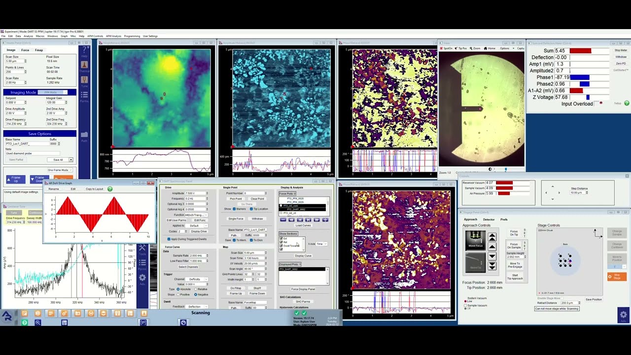
To start a downwards scan:

exp.execute('DownScan', wait=1.5)

2-4. Define a custom action based on a list of sequential operations

To start a scan with given save name and scan rate:

def ac_scan(self, scanrate, fname):
    action_list = [
        ['ChangeName', fname, None], # Change file names
        ['ScanRate', scanrate, None],# Change scan rate
        ['DownScan', None, 1.5],     # Start a down scan
        ['check_files', None, None], # Pause the workflow until number of files change in the save_folder 
    ]
    self.execute_sequence(operation=action_list)
    # Load the latest modified file in the data saving folder
    img = ae.ibw_read(ae.get_files(folder=self.folder)[0])
    return img

exp.add_func(ac_scan)

Then the custom action can be called in three ways:

# Preferred way: call it the same way as default actions
img = exp.execute('ac_scan', value=[1, 'NewImage'])

# Put it in the operation sequence list
action_list = [['ac_scan', [1, 'NewImage'], None], ['Stop', None, None]]
img = exe.execute_sequence(operation=action_list)

# Call as a method directly
img = exp.ac_scan(1, 'NewImage')

This is how a functional block is created.

2-5. Keep track of experiment parameters with exp.param dict

Let's store some useful parameters in the exp.param

# You can directly add it using exp.update_param()
exp.update_param(key='f_dart', value=353.125e3) # DART will tune the probe around this freq to make sure it can relibly track the resonance

# You can also update multiple parameters together:
p = {
    'v_dart': 1, # unit is V
    'f_width': 10e3, # Hz 
    'ScanSize': 5e-6, # um
    'ScanPixels': 256, # pixels
}
for key in p:
    exp.update_param(key=key, value=p[key])

This is particularly useful when you need to track many different data formats (list, np.ndarray, tensors) when integrating with machine learning algorithms.

2-6. Combinatorial library exploration

Link to the video of combinatorial exploration on a grid.

2-7. Deek Kernel Learning on Jupiter

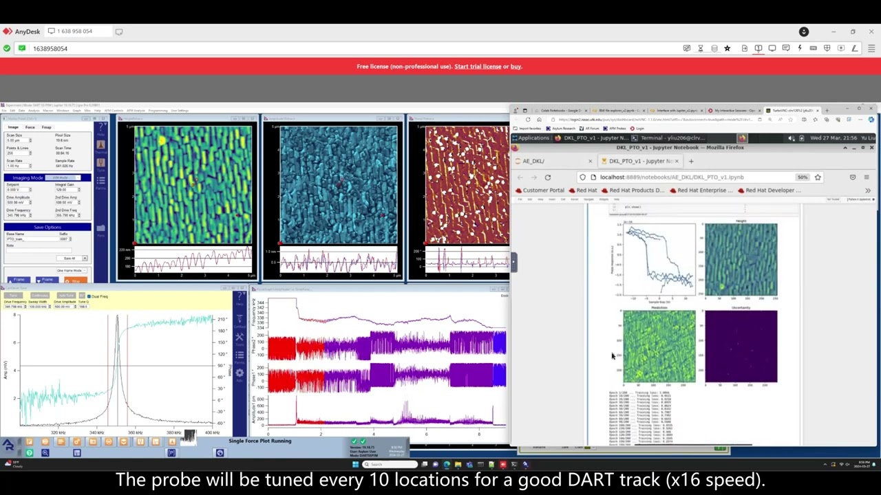
Link to the video of Deep Kernel active learning controlled from a supercomputer.

2-8. Autonomous optimization of SPM in the tapping mode

Link to the video of Deep Kernel active learning controlled from a supercomputer.

2-9 Variational Autoencoder to extract specific structures

3. Three levels of integration

3-1. spm_contrl()

The key function in the interface layer is spm_control(), which unifies the interaction with SPM controller.

spm_control() is a wrapper of lower-level write_spm() and read_spm(). It translates hyper-language actions that are familiar to users to instrument-specific codes/commands that controller can understand.

3-2. Experiment object

This is the fundamental object for AE workflows.

• exp.execute() calls spm_control() directly
• exp.execute_sequence() runs a list of actions in sequence
• exp.add_func() is the key to build functional blocks
• exp.param is a dict to keep track of experimental parameters and ML intermediate data
• It handles file I/O, SSH file transfer and connection automatically

3-3. Functional blocks and workflows

Functional blocks are defined based on a list of sequential actions that achieve one major task:

• Start an AC scan and load and plot the acquired image when it's done
• Move the probe to the location (x, y) and take a force-distance curve and extract final force when it's done.

These functional blocks can be created with Experiment.execute_sequence() and Experiment.add_func() methods. Once a functional block is appened to Experiment object, it can be called the same way as default single actions. Therefore, the full workflow can be built upon functional blocks, which makes it organized, concise, and easy to debug.

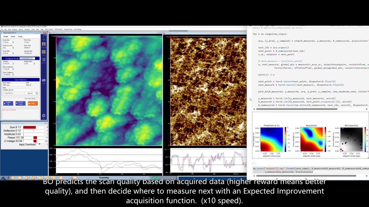
An example of AC exploration on a grid workflow build on functional blocks:

for i in range(num_points):
    print("Working on Location: {}/{}".format(i+1, num_points), end='\r')
   
    # Skip the first point
    if i:
        # Move the stage to the next grid point
        exe.execute('stage', value=[displacement])

    # AC scan
    exe.execute('start_ac_scan', value=['BSFO_AC{:03}_'.format(i+1)])