A Julia implementation of the Parareal algorithm from parallel-in-time integration using high-performance methods including GPU (e.g. CUDA.jl) and distributed (e.g. Distributed.jl) computing. The main aim of this work is to support the efficient simulation of equations of motion. Documentation can be found at https://nathanwchapman.com/PararealGPU.jl/dev/.
This work is not yet included in the Julia General Repository of packages as it is not yet completed. If you still want to tinker around with it, you can use Julia's package manager via
pkg> add https://github.com/NonDairyNeutrino/PararealGPU.jl
The Parareal algorithm (PA) comes from a class of algorithms dubbed parallel-in-time integration algorithms as their main goal is to accelerate the approximation of solutions to initial-value differential equations. The PA is one of the most widely studied methods in this class [1].
The key idea is that a single "root" initial value problem (IVP) can be broken into smaller IVPs using the data from an inaccurate "root" solution as the initial values of the subproblems. These subproblems are then solved in parallel using traditional, accurate methods. The final values of the resulting subsolutions are sequentially combined with those at the same time in the root solution to give a more accurate root solution. This process is then repeated until the root solution matches what would have ben obtained if the accurate method were used directly.
Because the PA leads to a quasi-pleasingly parallel set of problems that only need arithmetic operations to solve, the PA is well-suited to be implemented on massively parallel architectures such as GPUs, distributed systems, and supercomputers. The basic idea of the PA being executed on a single GPU is shown below, with an example cluster topology showing how the head node interacts with GPUs on remote machines; these images are sourced from my thesis, where this work was developed.

This implementation can be used to solve any problem you would traditionally, including the simple
harmonic oscillator. Here, nodeVector = String["Electromagnetism"] represents that the machine on
which this program is going to be executed can connect to a machine identified by "Electromagnetism"
via password-less ssh. The only information needed is these
ssh-identifiers; prepCluster automatically identifies and assigns all GPUs in the cluster
(including multiple GPUs in a single machine) to their own process.
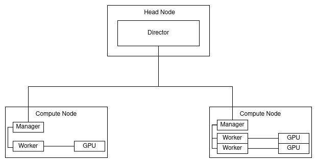
An example cluster topology is shown below. This cluster is composed of a head node, a compute node with one GPU, and a compute node with two GPUs. The head node is a machine that only has a single Julia process. This process is the "director" process that manages all other processes, and computes the sequential combination of the subsolutions and the root solution. The compute nodes have "middle manager" processes that manage the "worker" processes on the same machine; there is a worker process for every GPU in the machine.
using Plots
using PararealGPU
const nodeVector = String["Electromagnetism"]
devPool = prepCluster(nodeVector)

println("Creating initial value problems")
# DEFINE THE COARSE AND FINE PROPAGATION SCHEMES
const INITIALDISCRETIZATION = Threads.nthreads()
const COARSEPROPAGATOR      = Propagator(symplecticEuler, INITIALDISCRETIZATION)
const FINEPROPAGATOR        = Propagator(velocityVerlet,  2^0 * INITIALDISCRETIZATION)

@everywhere @inline function acceleration(position :: Vector{T}, velocity :: Vector{T}; k = 1) :: Vector{T} where T <: Real
    return -k^2 * position # this encodes the differential equation u''(t) = -k^2 u
end
const INITIALPOSITION = [0.]
const INITIALVELOCITY = [1.]
const DOMAIN          = Interval(0., 2^2 * pi)

ivpVector = Vector{SecondOrderIVP}(undef, length(devPool))
for k in 1:length(devPool)
    ivpVector[k] = SecondOrderIVP(DOMAIN, (x, v) -> acceleration(x, v; k), INITIALPOSITION, INITIALVELOCITY)
end

println("Beginning parareal evaluation on workers")
solutionVector = pmap(ivp -> parareal(ivp, COARSEPROPAGATOR, FINEPROPAGATOR), devPool, ivpVector)
println("Parareal evaluation finished")

for (k, rootSolution) in enumerate(solutionVector)
    plot!(
        rootSolution.domain,
        [rootSolution.positionSequence .|> first, rootSolution.velocitySequence .|> first],
        label = ["position - $k" "velocity - $k"],
        title = "discretization: $INITIALDISCRETIZATION    k <= $k"
    )
end
println("Plot saved at ", pwd(), "/cos.png")
savefig("cos.png")If you're still interested in learning more about the context surrounding this project, it was the central element of my master's thesis Scalable Parallel-in-Time Integration for Equations of Motion.