SAMRAI Data Reader
The hydrodynamics adaptive mesh refinement code HAMeRS, which is built on the SAMRAI library output vizualiztion data in the .samrai format. This tutorial illustrates how to read and post-process the viz data genrated from SAMRAI.
- use the serial SAMRAI data reader to read viz data generated from HAMeRS (using inviscid data generated from tutorial 5 in HAMeRS's wiki)
- read data on different grid levels
- read data upsampled to highest level in a sub-domain
- compute vorticity using a derivative class in FloATPy
"""
Import the modules
"""

from floatpy.readers import samrai_reader
import numpy

from matplotlib import pyplot as pltThe SAMRAI data reader requires the path to the "dumps.visit" during the initization. The "dumps.visit" has a list of visualization folders containing viz data corresponding to different time steps generated by SAMRAI. By default, the data is assumed to be be non-periodic and constant extraplotion is used during upsampling. However, user can change the default settings during the initialization of the data reader object. Here, we define the second dimension to be periodic, which is useful for getting ghost cells and also choose sixth order Lagrange interpolation as the upsampling method.
The first visualization dump is set as the current step during the initialization. The step can be changed after the reader is created.
# Get the SAMRAI serial data reader.
data_reader = samrai_reader.SamraiDataReader('./viz_2D_Richtmyer_Meshkov_instability/', \
                                            periodic_dimensions = (False, True), \
                                            upsampling_method = 'sixth_order_Lagrange')

# Get all the available steps to read and current step.
steps = data_reader.steps
print("All steps: %s" % steps)
print("Current step number: %s" % data_reader.step)

# Set the step number.
data_reader.step = steps[-1]
print("Current step number: %s" % data_reader.step)

# Print the simulation time of current step
print("Simulation time (s): %s" % data_reader.time)
All steps: [0, 73, 146, 219, 293, 367, 441, 515, 589, 663, 737, 811, 885, 959, 1033, 1107, 1181, 1255, 1329, 1403, 1478, 1553, 1628, 1703, 1778, 1853, 1928, 2003, 2078, 2153, 2228, 2303, 2378, 2453, 2528, 2603, 2678, 2753, 2828, 2903, 2978, 2979]
Current step number: 0
Current step number: 2979
Simulation time (s): 4e-05
The basic information such as the number of levels of grids, grid spacing of base grid, refinement ratios, variable names at the current step can be obtained from the method getBasicInfo().
basic_information = data_reader.getBasicInfo()
print(basic_information)
{'dim': 2, 'num_variables': 5, 't_dump': 'Wed Jan 31 22:44:20 PST 2018', 'ratios_to_coarser_levels': array([[-1, -1, 0],
[ 2, 2, 0],
[ 2, 2, 0]], dtype=int32), 'var_names': array(['pressure', 'sound speed', 'velocity', 'density', 'mass fraction 0'],
dtype='|S16'), 'n': 2979, 'x_lo': array([ 0., 0., 0.]), 'num_file_clusters': 8, 't': 4.0000000000000003e-05, 'dx': array([[ 3.12500000e-05, 3.12500000e-05, 0.00000000e+00],
[ 1.56250000e-05, 1.56250000e-05, 0.00000000e+00],
[ 7.81250000e-06, 7.81250000e-06, 0.00000000e+00]]), 'num_var_components': array([1, 1, 2, 1, 1], dtype=int32), 'num_patches': array([ 8, 21, 28], dtype=int32), 'num_levels': 3, 'grid_type': 'CARTESIAN', 'num_global_patches': 57}
The following steps are useful to get domain shape, coorainates and data at particular levels:
- domain shape at different grid levels can be found from
getDomainSizeAtOneLevel(level_number) - coordinates at different grid levels can be obtained from
getCoordinatesAtOneLevel(level_number) - load into the data reader by using
readDataAtOneLevel((tuple of variable names), level_number) - get data from the data reader with
getData(var_name)
Except the base level, data on higher grid levels are returned as a numpy array with size of a bounding box just large enough to contain data from all the patches at the requested level. As as results, data values at non-existing grid points at the requested grid level are represented by NaN's. In order to plot the data, the NaN values are better to be masked using numpy.ma.masked_where() first.
# Get the domain shapes.

domain_shape_0 = data_reader.getDomainSizeAtOneLevel(0)
domain_shape_1 = data_reader.getDomainSizeAtOneLevel(1)
domain_shape_2 = data_reader.getDomainSizeAtOneLevel(2)

print "Domain shape at first level: ", domain_shape_0
print "Domain shape at second level: ", domain_shape_1
print "Domain shape at third level: ", domain_shape_2

"""
Read and plot density data at base level.
"""

x_coords, y_coords = data_reader.getCoordinatesAtOneLevel(0)
data_reader.readDataAtOneLevel(('density',), 0)
rho = data_reader.getData('density')

X, Y = numpy.meshgrid(x_coords, y_coords)

plt.figure(figsize=(25, 2), dpi= 150)
plt.pcolormesh(X, Y, rho[:, :, 0].T)
plt.title('level 0', fontsize=16)
plt.xlabel('x (m)', fontsize=16)
plt.ylabel('y (m)', fontsize=16)
plt.show()

"""
Read and plot density data at highest level.
"""

x_coords, y_coords = data_reader.getCoordinatesAtOneLevel(2)
data_reader.readDataAtOneLevel(('density',), 2)
rho = data_reader.getData('density')

# Mask non-existing data (NaN).
rho_masked = numpy.ma.masked_where(numpy.isnan(rho), rho)

X, Y = numpy.meshgrid(x_coords, y_coords)

plt.figure(figsize=(20, 5), dpi= 150)
plt.pcolormesh(X, Y, rho_masked[:, :, 0].T)
plt.title('level 2', fontsize=16)
plt.xlabel('x (m)', fontsize=16)
plt.ylabel('y (m)', fontsize=16)
plt.show()
Domain shape at first level: (512, 32)
Domain shape at second level: (324, 64)
Domain shape at third level: (636, 128)


The SAMRAI data reader also provides the capability to load data in a sub-domain/chunk:
- set the sub-domain with the data reader property
sub_domain - get the coordinates in the sub-domain with
getCombinedCoordinatesInSubdomainFromAllLevels(num_ghosts) - load the data in the sub-domain into the data reader with
readCombinedDataInSubdomainFromAllLevels((tuple of variable names), num_ghosts) - data can be obtained from the data reader from
getData(var_name)
By default, the sub-domain shape is the full domain shape upsampled to the highest level. User can change the sub-domin with the data reader property sub_domain
print "Sub-domain shape upsampled to highest level: ", data_reader.sub_domain

# Set the sub-domain to be last 1/6 of the full domain.

domain_shape = data_reader.getRefinedDomainSize()
lo_subdomain = (domain_shape[0]*5/6, 0)
hi_subdomain = (domain_shape[0] - 1, domain_shape[1] - 1)

data_reader.sub_domain = (lo_subdomain, hi_subdomain)

print "Sub-domain shape upsampled to highest level: ", data_reader.sub_domain
Sub-domain shape upsampled to highest level: ((0, 0), (2047, 127))
Sub-domain shape upsampled to highest level: ((1706, 0), (2047, 127))
"""
Read density and velocity and plot density data upsampled at highest level in the sub-domain.
"""

x_coords, y_coords = data_reader.getCombinedCoordinatesInSubdomainFromAllLevels(num_ghosts=(0, 3))

data_reader.readCombinedDataInSubdomainFromAllLevels(('density', 'velocity'), num_ghosts=(0, 3))

rho = data_reader.getData('density')

X, Y = numpy.meshgrid(x_coords, y_coords)

plt.figure(figsize=(4, 2), dpi= 200)
plt.pcolormesh(X, Y, rho[:, :, 0].T)
plt.title('upsampled data', fontsize=12)
plt.xlabel('x (m)', fontsize=12)
plt.ylabel('y (m)', fontsize=12)
plt.show()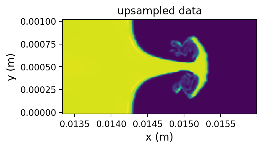
FloATPy also provides classes to compute derivatives. The cell below shows how to take curl on the velocity vector field to obtain the vorticity using the explicit derivative class.
# Load the explict differentiator class.
from floatpy.derivatives.explicit_differentiator import ExplicitDifferentiator

# Get the velocity data and compute the vorticity.

vel = data_reader.getData('velocity')

print "Shape of velocity data: ", vel.shape

dx = x_coords[1] - x_coords[0]
dy = y_coords[1] - y_coords[0]

explicit_diff = ExplicitDifferentiator((dx, dy), (6, 6), dimension=2, data_order='F')

vorticity = explicit_diff.curl(vel, use_one_sided=True)
vorticity = vorticity[:, 3:-3]

print "Shape of voriticity data: ", vorticity.shape

X, Y = numpy.meshgrid(x_coords, y_coords[3:-3])

plt.figure(figsize=(4, 2), dpi= 200)
plt.pcolormesh(X, Y, vorticity[:, :].T)
plt.title('vorticity', fontsize=12)
plt.xlabel('x (m)', fontsize=12)
plt.ylabel('y (m)', fontsize=12)
plt.show()
Shape of velocity data: (342, 134, 2)
Shape of voriticity data: (342, 128)
