This repository was created to host my favourite completed projects. Below I will give a brief summary and main insights of the projects. For further details please see the jupyter notebooks above.

Sea Turtle Face Detection with Distributed Machine Learning

The main goal of this project was to experiment with different options when trying to distribute ML training between workers on a cluster.

dask.org Dask is a python based API that facilitates distributed computing. It can link to a cluster of multiple workers and one scheduler computers. It provides multiple worflows to achieve distributed storing and manipulation of data. It is the main tool used in this project.

One options explored was using dask delayed to distribute a tensorflow CNN. The other option explored was using a scikit learn MLP classifier which is completly dask supported.

Computational Time Line Comparison

Dask Delayed Distribution of a Tensorflow CNN (5 epochs)

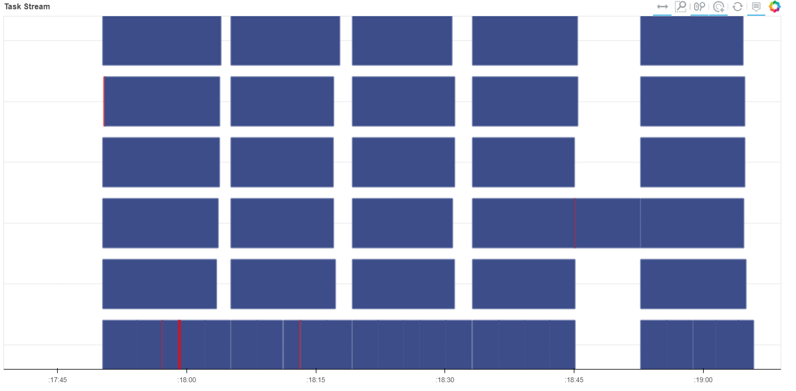
Dask Distribution of a scikit learn MLP classifier (1 epoch)

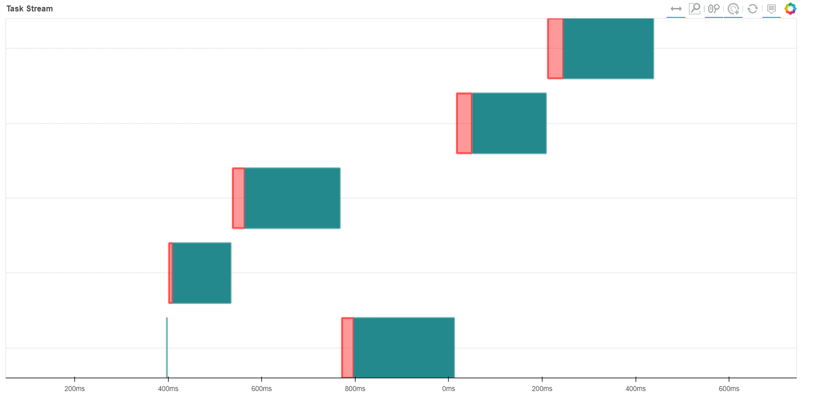
Each row in the images above represents a worker on the cluster. The red color indicates that information is being transfered from another worker. The other colors represent a task pering performed by the worker. Time is on the x axis. You can see that when dask distributes the MLP classifier it does not train in paralell. Each worker will train on the data it has collected and then transfer the weights to the next worker to continue training. This strategy will allow the system to break through memory limitations. Although this system does not help reduce training time. The custom dask delayed distribution of the tensorflow CNN is a stark contrast. It will train in paralell. This could potentially lead to reduced training times for large datasets. The data is also split between the workers allowing to break memory limitations. For the small dataset of 4000 198x198 images the paralell training of the dask delayed CNN did not cause faster training times than the unparalell supported MLP. One epoch took 10min for the CNN and only 1 second for the MLP. This is partially because the MLP is a simpler algorithm that was fed further processed HOG versions of the images. The CNN is a more complex algorithm with more weights to alter and is fed the full color images. It is also partially due to the MLP being dask supported and thus optimised. Dask themselves admit that whilst dask delayed is flexible it is also slow.

Investigation of Binary Black Hole Properties and their Effect on Time Delay

Time delay is the time gap between the formation of a binary star system and their merging. The project focused on systems that became binary black before merging. The investigation was to discern which properties of the systems has the most affect on time delay. Firstly the relationships are analysed graphically. Then XGBoost and Decision tree regression algorithms were trained to predict time delay given system properties. These can output which properties had the greatest effect on its decision.

Graphical Analysis Example

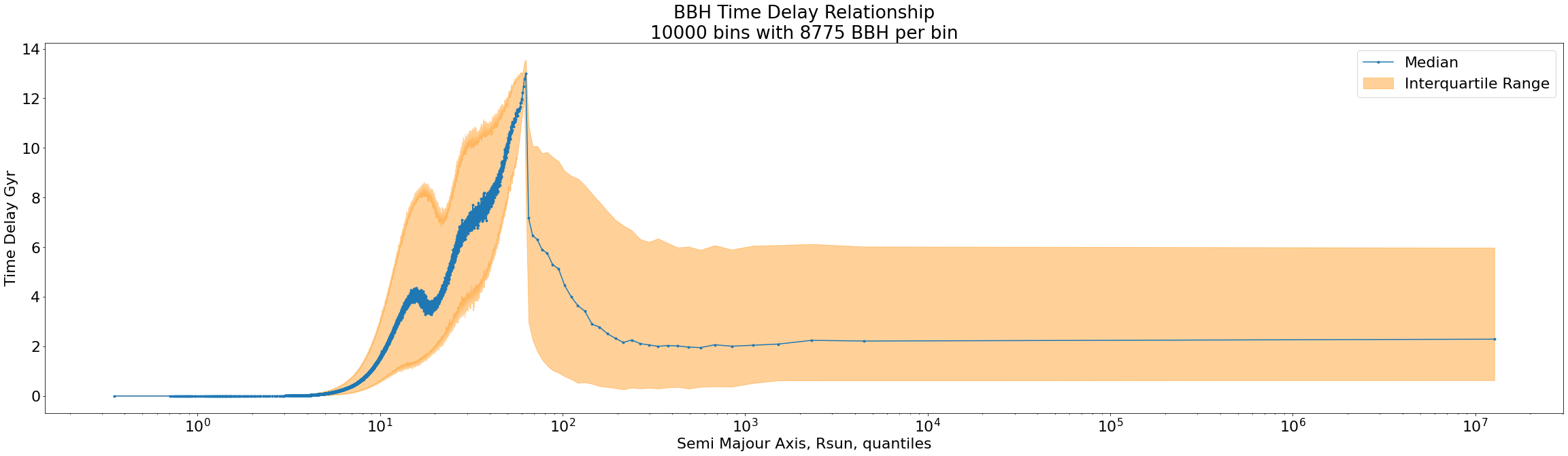The semi majour axis is effectivly the distance between the two objects in the binary system when formed. The graph includes $8 \cdot 10^7$ black holes that are divided into bins that all include the same number of black holes but have different values of the semi majour axis. As the graph is feature rich we can summise that the semi majour axis has a strong effect on the time delay. One would assume that if the binary objects are far apart when the system is formed (semi-mjr axis) then the time taken to merge (time delay) should be large. This general logic holds true except for exceptionally large semi majour axis values. This is after the the peak in the graph above where the trend flat lines. The study continues to show that these systems are also the systems that have the most ideal mass's and common envalope efficiencies for a short time delay.

XGBoost Regression Example

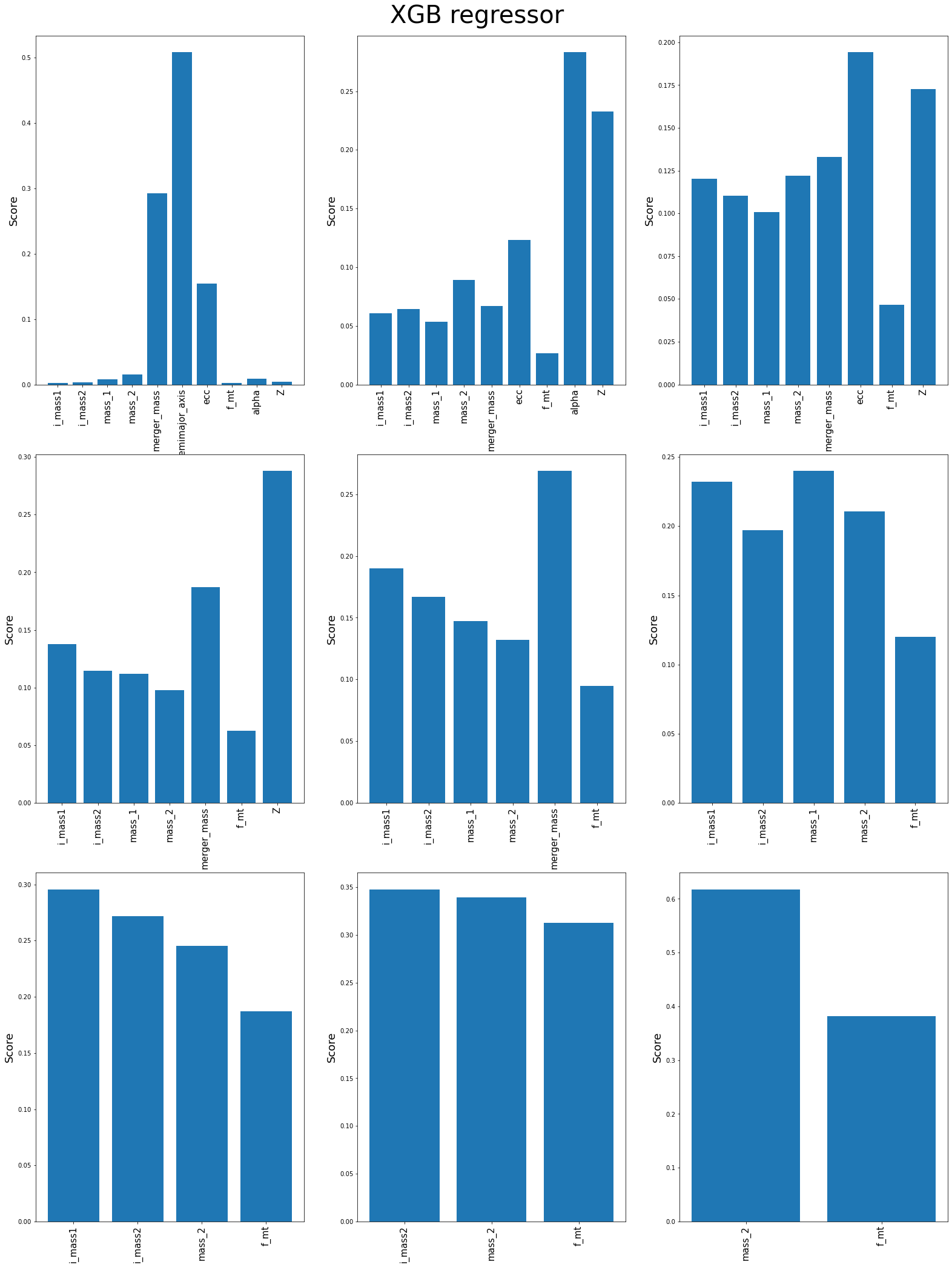
The XGBoost algorithm was trained to predict the time delay of the binary black holes given the properties of the black hole. It can also output the importances of each property to its decisions. The graph above shows these importances. Going from left to right top to bottom you can see a progression of the graphs. At each step in the progression the most important feature from the previous graph is removed. The top three properties that affect time delay is the semi majour axis, common envalope efficiency (alpha) and orbital eccentricity (ecc). In the graphical approach both common envalope efficiency and semi majour axis showed some distinct features and trends. Although orbital escentricity did not. It was mostly a flat line. Thus this finding was unexpected. The high dimensionality of the data means that such trends are over simplified when only looking at a 2D graph. The machine learning approach was likly able to find a true trend where the grpahical approach failed.

Optimisation of Interferometry Lines of Sight for Future Nuclear Fusion Experiments with the Bayesian Experimental Design Framework

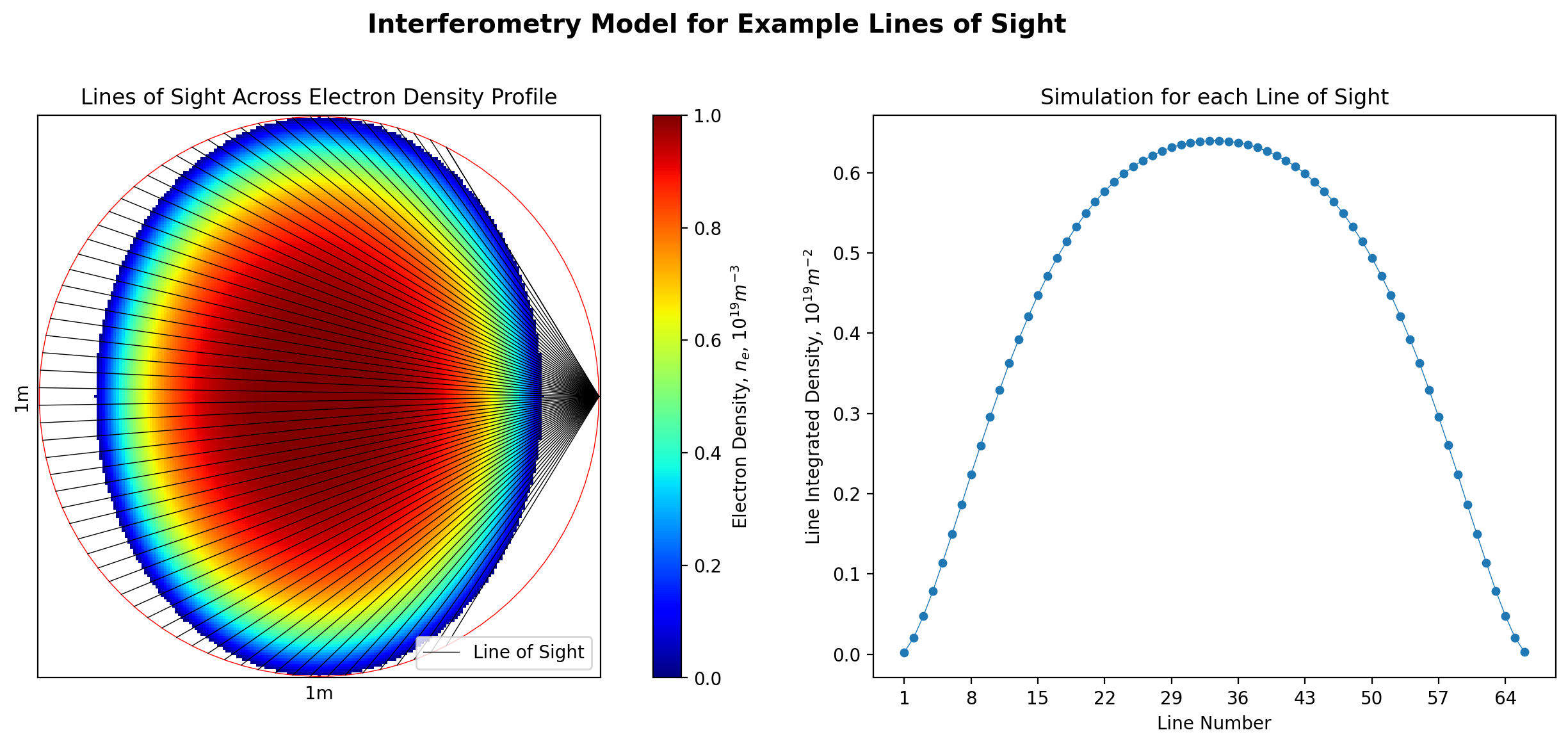The left of the plot shows a model plasma density inside a pollodial cross section of a tokamak. The plasma density is constant at magnetic field lines. The black lines represent interferometry lasers. The start angle is kept fixed while the end angle is altered. The plot on the right shows simulated line integrated densities that the interferometry would be aiming to measure.

Bayesian experimental design uses the KL-divergence between the prior and posterior probability distribution associated with a physical parameter of interest. Interferometry aims to measure the plasma density profile across the cross section of a tokamak. The prior distribution represents our knowledge of the plasma density profile before the experiment and the posterior our knowledge after the experiment. The KL-divergence is the information gain from the experiment. Multiple experiments can be simulated with different design parameters to estimate the design parameters that lead to the most information gain. In this investigation the orientation of interferometry lasers is the design parameter that is altered.

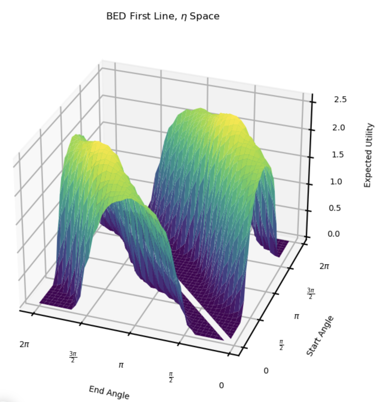
The above plot shows the estimated expected utility surface. The expected utility is defined as the expected KL-divergence over all possible data measurements. It is calcuated for interferometry experiments with one laser at different orentations. Each orientation is a different point on the surface. The orientation is defined by a start and end angle. The ridge corrosponds to lines through the center. These reach a maximum when the line is also vertically orientated. With start and end angles of $\frac{\pi}{2}$ and $\frac{3\pi}{2}$. The symetry occures because when start and end angles are flipped the orientation is the same and so the expected utlitiy is the same. To conclude, for this plasma model the line of sight that gives the maximum potential for information gain is the vertical line through the center with angles $\frac{\pi}{2}$ and $\frac{3\pi}{2}$.