Optics Module

The optics module calculates the spectrally and angular-resolved absorptance for a variety of different architectures of single or multi-junction solar cells. It is able to handle multiple planar and textured interfaces with coherent and incoherent light propagation by combining the transfer matrix method (TMM) and geometrical ray-tracing.

First, the defined architecture is analyzed and divided into optically thin (coherent) partial stacks and optically thick (incoherent) layers. In this regard, a coherent layer stack is defined by two incoherent boundary layers. The light propagation and absorption in any incoherent layer separating two of such partial stacks is treated with the Beer-Lambert law, with which the absorption is calculated. For multiple adjacent incoherent layers, the transmittance and reflectance at their interfaces are calculated with the Fresnel equations.

For each partial stack and for each incoherent layer the reflectance, transmittance and absorption in forward and in backward direction are determined. All these quantities are spectrally resolved.

In order to calculate the total reflectance, transmittance and the absorptance in each layer, these quantities are connected by subsequently adding partial stacks or incoherent layers. A simple example is illustrated in the figure. Here, two partial stacks consisting of 3 and 4 coherent layers are connected. The properties: reflectance R and transmittance T for the coherent layers and the absorptance A for the coherent layers for light propagating in forward and backward direction are shown. In addition, the absorptance A_inc in the incoherent layer is shown, at which the stacks are merged.

First, reflectance is derived by following the ray interactions (see above figure) within the joined stack. The total reflectance is then the sum over the individual paths:

Where we use the following abbreviation:

Next, the transmittance is derived in an analogous way, which leads to:

Finally, the absorptance is calculated. Here, three cases need to be distinguished. The absorptance in the coherent layers of the first partial stack (=top):

the absorptance of the incoherent layer connecting the two partial stacks:

and the absorptance in the coherent layers of the second partial stack (=bottom):

The advantage of this approach is, that for each of the incoherent layers, defined within the full stack, it is possible to add a texture. The texturing can be done by setting the morphology for each incoherent layer. The texturing then is added at the interface between this incoherent layer and the above layer(s) / layer stack. In the above architecture with 3 incoherent layers, texturing the last (3) incoherent layer will lead to the following scenario:

Note: since texturing of the first (1) incoherent layer facing upwards makes no sense, the input of the morphologies start at the second (2) layer: e.g. {‘Flat’, ‘Texture‘}.

In order to use a specific texture, either the redistribution matrices for R, A and T need to be a known property. Or they will be calculated by the use of path data extracted from OPAL2.

The geometrical ray-tracing as described by Baker-Finch and McIntosh is an elegant approach that allows fast calculation of the characteristic paths for textures (e.g., pyramids). This gives us a limited set of paths with its probabilities and their intersection angles.

Usage

First, we define the input parameters and call the optics analogous to the description in the quick start guide.

Stack = {'Air','MgF2','Glass1.5','ITOfront','SnO2','Pero1.62','SpiroOMeTAD',...
    'ITOfront','aSi(n)','aSi(i)','cSi','aSi(i)','aSi(p)','ITOfront','Air'};
LayerThickness = [inf,100,1E4,100,10,450,20,25,5,5,250E3,5,5,100,inf];
Morphology = {'Flat','RandomUpright','RandomUpright'};
Polarization = 'mixed';
lambdaTMM = 300:5:1200;  
AngleResolution = 5;
IncoherentLayers = {'Air','Glass','cSi'};
bifacial = false;
Absorbers = {'Perovskite','cSi'};

optics = OpticsModule(IndRefr, Stack, LayerThickness, AngleResolution, Morphology, bifacial, Polarization, lambdaTMM, PathOpticsResults, StoreInDatabase, IncoherentLayers, Absorbers);

This gives us a struct called optics, which contains the interesting quantities:

>> optics

optics = 

  struct with fields:

      Reflectance: [90×90×181 single]
      Absorptance: [13×90×181 single]
    Transmittance: [90×181 single]
           lambda: [1×181 double]
    AbsorberIndex: [5 10]
                A: [181×2 single]
                R: [181×1 single]
                T: [181×1 single]
             hash: "DCCC4EDAAA22C57CFDEA5578ADA460A744DBE13F"

Reflectance and Transmittance are given as tensors of dimension: [angle of incidence x angle of escape x wavelength]. The dimension of the Absorptance matrix is [number of layer x angle of incidence x wavelength]. In addition, those quantities are also provided for normal incidence only and summed up for all escape angles: A, R, and T. Moreover, the absorption is only given for the absorbers.

We can plot this:

Aall = squeeze(sum(optics.Absorptance(:,1,:)));	% get total absorptance

figure; 
plot(lambdaTMM, optics.A );hold on
plot(lambdaTMM, optics.R );
plot(lambdaTMM, optics.T ); 
plot(lambdaTMM, Aall,'--');hold off
xlabel('Wavelength (nm)'); ylabel('R, A, T')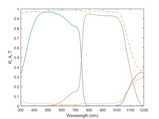

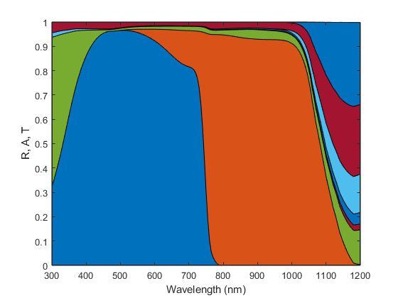
A = squeeze(optics.Absorptance(optics.AbsorberIndex,1,:))';
Aparasitic = squeeze(optics.Absorptance(setdiff(1:size(optics.Absorptance,1),optics.AbsorberIndex),1,:))';

figure;
area(lambdaTMM, [A, Aparasitic, optics.R, optics.T] );
xlabel('Wavelength (nm)'); ylabel('R, A, T')