DAISIErobustness R package
-
Rpackage
DAISIErobustness main feature consists of a pipeline designed to measure the error one creates when extending the standard DAISIE model with new features. Examples of such new additions include the modelling of island ontogeny, as per the General Dynamic Model3, sea level changes4, and continental scenarios. The error measure is obtained by simulating and comparing DAISIE data using simulation code that builds upon the existing DAISIE simulations by including geodynamic processes.
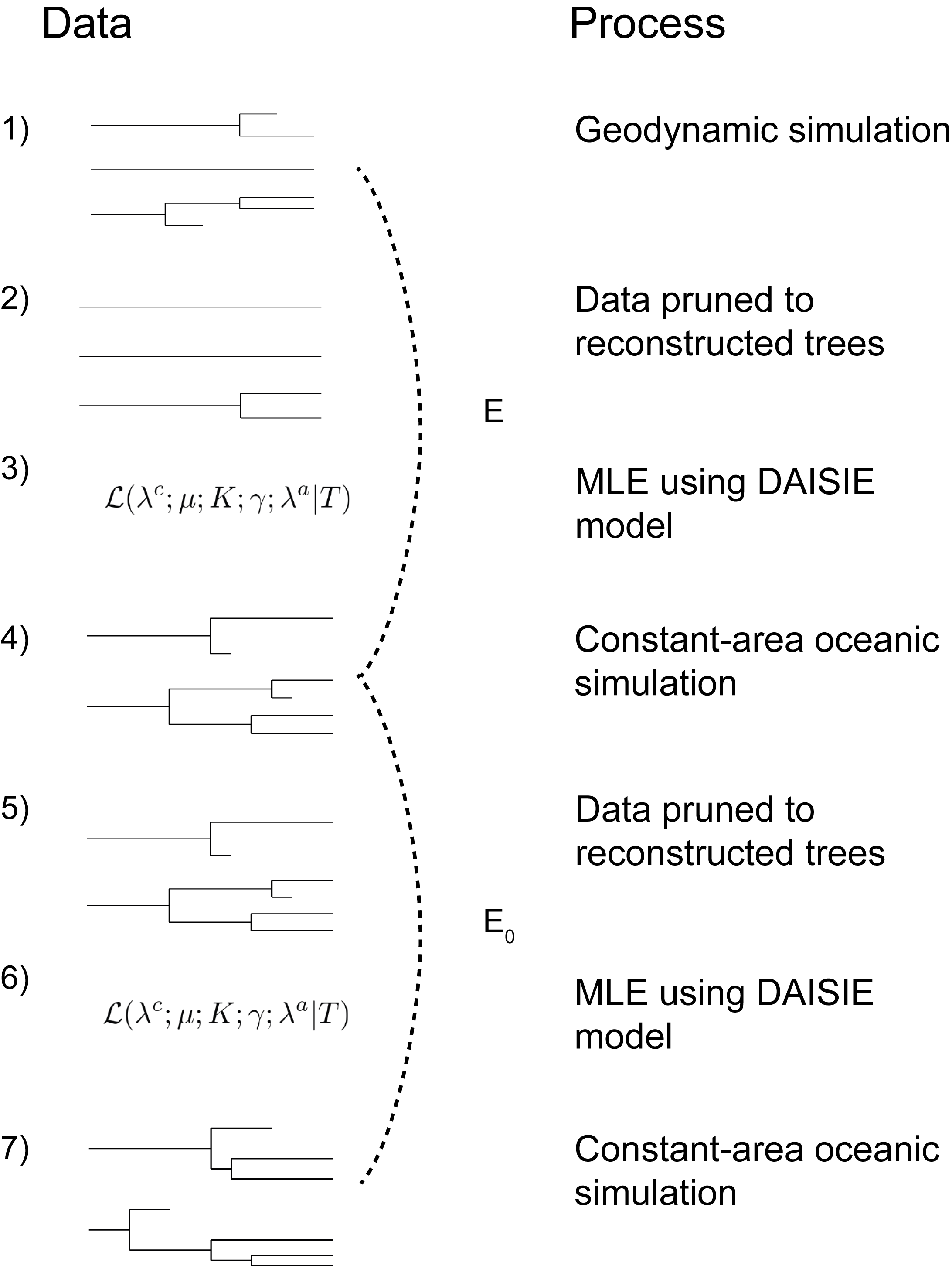 Schematic representation of the robustness pipeline.
- Island phylogenetic data is produced by a geodynamic simulation.
- Reconstructed phylogenetic data is produced by pruning (removing) all extinct lineages.
- DAISIE maximum likelihood estimation (MLE) of parameters, which assumes no geodynamics, is applied to data from step 2.
- A constant-area oceanic simulation (i.e. the original DAISIE method) is run with the parameters estimates from step 3 as generating parameters.
- Phylogenies are pruned to reconstructed trees.
- The DAISIE MLE is applied to data from step 5.
- A constant-area oceanic simulation is run with parameter estimates from step 6 as generating parameters. The inference error made on data from a geodynamic simulation (E, step 3) is compared with the baseline error (E0, step 6). The error E is calculated by comparing the geodynamic simulations with the first set of constant-area oceanic simulations for five metrics (dashed line). The baseline error E0 is obtained by comparing two oceanic simulations using the same five metrics (dashed line). The error made when inferring from geodynamic data but assuming the constant-area oceanic model in inference is the proportion of errors (E) that exceed the 95th percentile of the baseline errors (E0).
Several inbuilt models are included in the DAISIErobustness
run_robustness(). The parameter space and models this function can accept are stored in the /inst/extdata folder, and were generated by running the generate_param_space.R script. The available parameter spaces are:
- Continental:
continental - Continental with land bridges:
continental_land_bridge - Continental with sea-level changes:
continental_sea_level - Oceanic ontogeny:
oceanic_ontogeny - Oceanic ontogeny with sea-level changes:
oceanic_ontogeny_sea_level - Oceanic with sea-level changes:
oceanic_sea_level - Trait dependency:
trait
The codes in mono-spaced font serve as arguments for the run_robustness() function. Then, the corresponding csv parameter space is read from the GitHub repository to the function scope, so that the pipeline can begin.
run_robustness(
   param_space_name = "oceanic_ontogeny_cs",
   param_set = 1,
   replicates = 10,
   distance_method = "abs",
   save_output = TRUE
  )
This code will start the pipeline for the first parameter set in the oceanic ontogeny clade-specific parameter space. The first parameter set corresponds to the first line in the matching data file. 10 oceanic ontogeny clade-specific pipeline replicates will run.
When save_output = TRUE, all the objects generated by the pipeline will be stored in the package's root folder (or the session's working directory, as set by setwd() if such is done), into /results/param_space_name, param_space_name corresponding to parameter spaced given when the function is called. These directories will be created if not present and if write permissions allow.
If save_output = FALSE, then the objects will be returned by the function, allowing them to be saved to an R object and handled in an interactive session.
The parameter currently implemented can be found here. New parameter sets can be generated using this helpful script.
The following results are used to determine the error between models:
- The nLTT5 statistic for endemic species, non-endemic species and all species.
- The difference at the end of the simulation of the number of species, endemic and nonendemic species.
These metrics are then aggregated between all replicates of a given parameter space in the following way:
- Mean and standard deviation in the difference of all nLTTs
- Mean and standard deviation of number of species, endemics and nonendemics
Given the stochastic nature of the simulation models, and that given the very nature of these studies the properties of the simulated output are not known, some constraints must be made on the simulated data and likelihood estimates. When the data generated by a simulations of a certain parameter space does not respect the constraints, these data are saved (to the degree they are generated) but not analysed.
The code used to generate the figures found in the REFREFREF paper can be found in the ´/scripts/plots/´ directory. Functions that generate the figures are found within the /functions/ sub-directory, while the scripts that load, plot and save the files are found in the root of the /plots/ directory. How to load files, and download files.
3Whittaker, Robert J., Kostas A. Triantis, and Richard J. Ladle. "A general dynamic theory of oceanic island biogeography." Journal of Biogeography 35.6 (2008): 977-994.
4Fernández‐Palacios, José María, et al. "Towards a glacial‐sensitive model of island biogeography." Global Ecology and Biogeography 25.7 (2016): 817-830.
5Janzen, Thijs, Sebastian Höhna, and Rampal S. Etienne. "Approximate Bayesian Computation of diversification rates from molecular phylogenies: introducing a new efficient summary statistic, the nLTT." Methods in Ecology and Evolution 6.5 (2015): 566-575.