Artefact in map #76
Description
Hey,
I have a problem and I can't fix it on my own. I'm trying to create a gift for someone and I want to plot a 60min radius of certain cities and places.
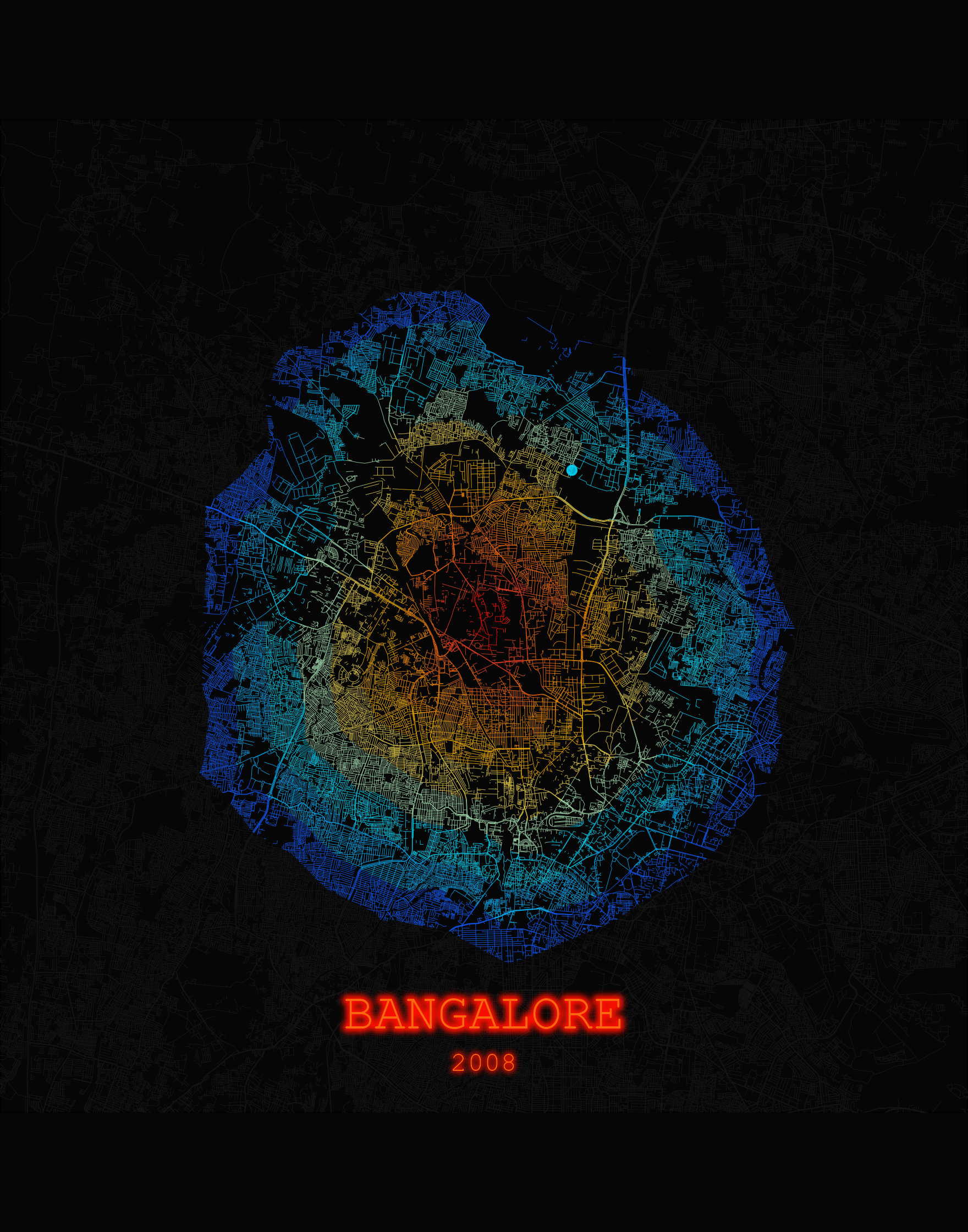
For the map in Bangalore, I get a strange circle artifact and I fail to identify it in my data. I would love the map without the round circle in it.
By looking at the online isochrones and google maps I can't see anything that could explain the circle in my plot below. I tried to comment on my code, but it might be very basic for most of you.
Any help would be highly appreciated!
Cheers,
Sven


Here is my code - should work for you
#load packages  -------------------
library(openrouteservice)
library(mapview)
library(tidyverse)
library(osmdata)
library(sf)
library(paletteer)
library(ggfx)
ors_api_key("my_functioning_api_key")
coordinates <- data.frame(lon = c(77.56373409967735), lat = c(13.023577094186736))
#creating intervals for a 60-minute walk from the starting point [coordinates]
cj_iso <- ors_isochrones(locations = coordinates, profile = "foot-walking",
range = 6000, interval = 600, output = "sf")
intervals <- levels(factor(cj_iso$value))
cj_iso_list <- split(cj_iso, intervals)
cj_iso_list <- cj_iso_list[rev(intervals)]
#creating new names for the lists
names(cj_iso_list) <- sprintf("%s_min", as.numeric(names(cj_iso_list))/60)
#check if everything looks good
# mapviewOptions(fgb = FALSE)
#mapview(cj_iso_list, alpha.regions = 0.2, homebutton = FALSE, legend = FALSE)
#min max data frame for coordinates
x <- c(coordinates$lon - 0.1, coordinates$lon + 0.1)
y <- c(coordinates$lat - 0.1, coordinates$lat + 0.1)
custom_wandsworth <- rbind(x,y)
colnames(custom_wandsworth) <- c("min", "max")
#extracting streets to sf()
streets <- custom_wandsworth %>%
opq() %>%
add_osm_feature(key = "highway",
value = c("motorway", "primary",
"secondary", "tertiary",
"trunk", "secondary_link", "tertiary_link",
"residential", "living_street",
"unclassified",
"service",
"footway",
"bicycle_road" )) %>%
osmdata_sf()
#function to get the geometry and the streets in one place
rep.x <- function(i, na.rm = FALSE) {
if(i == length(cj_iso_list)) {streets$osm_lines %>% st_intersection(cj_iso_list[[i]])}
else if(i < length(cj_iso_list)) {streets$osm_lines %>% st_intersection(st_difference(cj_iso_list[[i]], cj_iso_list[[i+1]]))}
}
list_df <- lapply(1:length(cj_iso_list), rep.x)
iso_df <- dplyr::bind_rows(list_df)
#funny color palette
colpal = fish(10, option = "Hypsypops_rubicundus") %>%
  prismatic::color()

#annotatitons for the map
hflat <- "BANGALORE"
hyar <- "2008"


#plotting with ggplot
ggplot() +
  geom_sf(data = streets$osm_lines,
          color = "#151515",
          linewidth = .1) +
  geom_sf(data = iso_df,
          aes(colour = as.factor(value),
              geometry = geometry),
          fill = "#060606",
          linewidth = .1,
          alpha = .8) +
  scale_colour_manual(values = rev(colpal))+
  coord_sf(xlim = custom_wandsworth[1,],
           ylim = custom_wandsworth[2,],
           expand = FALSE)  +
  ggfx::with_outer_glow(annotate(geom = "text", label = hflat,
           x = coordinates$lon, y = custom_wandsworth[2,1]+.02,
           size = 7.5, hjust = 0.5, colour = colpal[8], family = "mono"),
           colour = colpal[10], sigma = 5, expand = 7) +
  ggfx::with_outer_glow(annotate(geom = "text", label = hyar,
           x = coordinates$lon, y = custom_wandsworth[2,1]+.01,
           size = 4, hjust = 0.5, colour = colpal[8], family = "mono"),
           colour = colpal[10], sigma = 5
           , expand = 3) +
  theme_void() +
  guides(color = "none") +
  theme(plot.background = element_rect(fill = "#060606"),
        panel.background = element_rect(fill = "#060606"))

ggsave(filename = paste0("henrik_",hflat,"_", format(Sys.time(), "%d%m%Y"), ".png"),
       plot = last_plot(),
       dpi = 320,
       width = 5.5,
       height = 7)